Creating a PM function

We’ll go through the steps of creating the P50 function.

First, we create a new object of class PMobj, and populate the Name slot with a short but descriptive name:

PMobj <- new("PMobj")
PMobj@Name <- "Spawning Biomass relative to SBMSY"

The next line populates the Caption slot with a brief caption including the years over which the performance statistic is calculated. The if statement is not crucial, but avoids the redundant SB > 1 SBMSY in cases where Ref=1.

Next we store the value of the Ref argument in the PMobj@Ref slot so that information is contained in the function output.

PMobj@Ref <- Ref

The Stat slot is an array that stores the variable which we wish to calculate the performance statistic; an output from the runMSE function with dimensions MSE@nsim, MSE@nMPs, and MSE@proyears (or fewer if the argument Yrs != NULL).

In this case we want to calculate a performance statistic related to the biomass relative to BMSY, and so we assign the Stat slot as follows:

PMobj@Stat <- MSEobj@SB_SBMSY[, , Yrs[1]:Yrs[2]]

Note that we are including all simulations and MPs and indexing the years specified in Yrs.

Next we use the calcProb function to calculate the mean of PMobj@Stat > PMobj@Ref over the years dimension. This results in a matrix with dimensions MSE@nsim, MSE@nMPs:

PMobj@Prob <- calcProb(PMobj@Stat > PMobj@Ref, MSEobj)

Note that in order to calculate a probability the argument to the calcProb function must be a logical array, which is achieved using the Ref slot.

Also note that in this case PMobj@Stat > PMobj@Ref is equivalent to MSEobj@SB_SBMSY[, , Yrs[1]:Yrs[2]] > 0.5.

The PM functions have been designed this way so that in most cases the PMobj@Prob <- calcProb(PMobj@Stat > PMobj@Ref) line is identical in all PM functions and does not need to be modified. The exception to this is if we don’t want to calculate a probability but want the actual mean values of PMobj@Stat, demonstrated in the example below.

In the next line we calculate the mean of PMobj@Prob over simulations using the calcMean function:

PMobj@Mean <- calcMean(PMobj@Prob)

Similar to the previous line, this line is identical in all PM functions and can be simply copy/pasted from other PM functions without being modified. The Mean slot is a numeric vector of length MSEobj@nMPs with the overall performance statistic, in this case the probability of \(\text{SB} > 0.5\text{SB}_\text{MSY}\) across all simulations and years.

Finally, we store the names of the MPs and return the PMobj.

Creating Example PMs and Plot

As an example, we will create another version of DFO_plot using some custom PM functions and a customized version of TradePlot.

First we create the plot using DFO_plot:

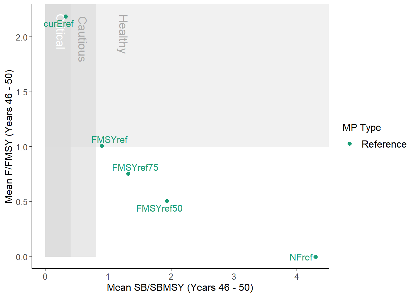
DFO_plot(MSEobj)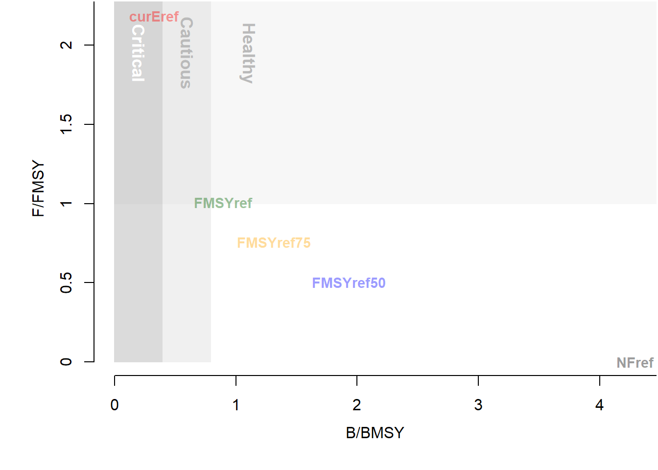

From the help documentation (?DFO_plot) we can see that this function plots mean spawning biomass relative to \(\text{SB}_\text{MSY}\) and fishing mortality rate relative to \(F_\text{MSY}\) over the final 5 years of the projection.

First we’ll develop a PM function to calculate the mean \(\text{SB}_\text{MSY}\) for the last 5 years of the projection period. Notice that this is very similar to P50 described above, with the modification of the Caption and the Prob slots, and the Yrs argument. We are calculating a mean here instead of a probability and are not using the Ref argument:

MeanB <- function(MSEobj = NULL, Ref = 1, Yrs = -5) {
    Yrs <- ChkYrs(Yrs, MSEobj)
    PMobj <- new("PMobj")
    PMobj@Name <- "Spawning Biomass relative to SBMSY"
    PMobj@Caption <- paste0("Mean SB/SBMSY (Years ", Yrs[1], " - ", Yrs[2], ")")
    PMobj@Ref <- Ref
    PMobj@Stat <- MSEobj@SB_SBMSY[, , Yrs[1]:Yrs[2]]
    PMobj@Prob <- calcProb(PMobj@Stat, MSEobj)
    PMobj@Mean <- calcMean(PMobj@Prob)
    PMobj@MPs <- MSEobj@MPs
    PMobj
}

We develop a PM function to calculate average F/FMSY in a similar way:

MeanF <- function(MSEobj = NULL, Ref = 1, Yrs = -5) {
    Yrs <- ChkYrs(Yrs, MSEobj)
    PMobj <- new("PMobj")
    PMobj@Name <- "Fishing Mortality relative to FMSY"
    PMobj@Caption <- paste0("Mean F/FMSY (Years ", Yrs[1], " - ", Yrs[2], ")")
    PMobj@Ref <- Ref
    PMobj@Stat <- MSEobj@F_FMSY[, , Yrs[1]:Yrs[2]]
    PMobj@Prob <- calcProb(PMobj@Stat, MSEobj)
    PMobj@Mean <- calcMean(PMobj@Prob)
    PMobj@MPs <- MSEobj@MPs
    PMobj
}

Similar to developing custom MPs we need to tell R that these new functions are PM methods:

class(MeanB) <- "PM"
class(MeanF) <- "PM"

Now we can test our performance metric functions:

data.frame(MP=MeanB(MSEobj)@MPs, 
           SB_SBMSY=MeanB(MSEobj)@Mean, 
           F_FMSY=MeanF(MSEobj)@Mean)

##          MP  SB_SBMSY       F_FMSY
## 1   curEref 0.3258801 2.186392e+00
## 2   FMSYref 0.8950520 1.008874e+00
## 3 FMSYref50 1.9335515 5.044369e-01
## 4 FMSYref75 1.3170624 7.566554e-01
## 5     NFref 4.2925589 4.017549e-15

How do these results compare to what is shown in DFO_plot?

We could also use the summary function with our new PM functions, but note that these results are not probabilities:

summary(MSEobj, 'MeanB', 'MeanF')

## Calculating Performance Metrics

##                  Performance.Metrics                               
## 1 Spawning Biomass relative to SBMSY  Mean SB/SBMSY (Years 46 - 50)
## 2 Fishing Mortality relative to FMSY    Mean F/FMSY (Years 46 - 50)
## 
## 
## Performance Statistics:
##          MP MeanB   MeanF
## 1   curEref  0.33 2.2e+00
## 2   FMSYref  0.90 1.0e+00
## 3 FMSYref50  1.90 5.0e-01
## 4 FMSYref75  1.30 7.6e-01
## 5     NFref  4.30 4.0e-15

Finally, we will develop a customized plotting function to reproduce the image produced by DFO_plot.

We can produced something fairly similar quite quickly using the TradePlot function:

TradePlot(MSEobj, 'MeanB', 'MeanF', Lims=c(0,0))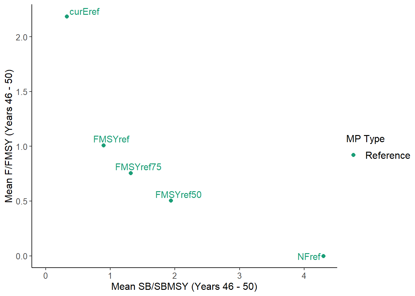

##          MP MeanB   MeanF Satisificed
## 1   curEref  0.33 2.2e+00        TRUE
## 2   FMSYref  0.90 1.0e+00        TRUE
## 3 FMSYref50  1.90 5.0e-01        TRUE
## 4 FMSYref75  1.30 7.6e-01        TRUE
## 5     NFref  4.30 4.0e-15        TRUE

Adding the shaded polygons and text requires a little more tweaking and some knowledge of the ggplot2 package. We will wrap up our code in a function:

NewPlot <- function(MSEobj) {
  # create but don't show the plot
  P <- TradePlot(MSEobj, 'MeanB', 'MeanF', Lims=c(0,0), Show='none') 
  P1 <- P$Plots[[1]] # the ggplot objects are returned as a list
  
  # add the shaded regions and the text
  P1 <- P1 + ggplot2::geom_rect(ggplot2::aes(xmin=c(0,0,0), xmax=c(0.4, 0.8, Inf), 
                                       ymin=c(0,0,1), ymax=rep(Inf,3)),
                          alpha=c(0.8, 0.6, 0.4), fill="grey86") +
    ggplot2::annotate(geom = "text", x = c(0.25, 0.6, 1.25), y = Inf, 
                      label = c("Critical", "Cautious", "Healthy") , 
                      color = c('white', 'darkgray', 'darkgray'), 
                      size=5, angle = 270, hjust=-0.25)
  
  # Re-order layers so text and points are not covered
  P1$layers <- c(P1$layers, P1$layers[[3]], P1$layers[[4]])
  P1$layers[[3]] <- P1$layers[[4]] <- NULL
  P1
}

NewPlot(MSEobj)