Add Data to OM

To condition our OM with catch data, we create a blank Data object:

Data <- new('Data')

and populate the Year, Cat, and CV_Cat slots with our observed data:

# years - must be length(OM@nyears)
Data@Year <- RealData@Year 

# 'real' catches (can be patchy)
Data@Cat <- RealData@Cat[1,,drop=FALSE] 

# assumed CV=0.2 all years
Data@CV_Cat <- matrix(0.2, nrow=1, ncol=length(Data@Year))

and add the Data object to the cpars slot:

OM <- new('OM', Albacore, Generic_IncE, Generic_Obs, Perfect_Imp, nsim=4)
OM@cpars$Data <- Data

Condition Catch Observation Model

The observation model is conditioned on the catch data when the historical spool-up period is simulated:

Hist <- Simulate(OM, silent=TRUE)

We can now compare our simulated catch with our ‘real’ observed catches:

# The catch data that are passed to the MPs
ObsCatches <- Hist@Data@Cat

# first 5 years of the 'real' catch data
OM@cpars$Data@Cat[1,1:5]

## [1]   82.33424  272.39243 1151.69521 1209.50230  938.61773

# first 5 years of simulated 'observed' catch data passed to MPs
ObsCatches[,1:5]

##          [,1]     [,2]     [,3]     [,4]     [,5]
## [1,] 82.33424 272.3924 1151.695 1209.502 938.6177
## [2,] 82.33424 272.3924 1151.695 1209.502 938.6177
## [3,] 82.33424 272.3924 1151.695 1209.502 938.6177
## [4,] 82.33424 272.3924 1151.695 1209.502 938.6177

# first 5 years of catch data simulated from OM
Catches <- apply(Hist@TSdata$Landings, 1:2, sum) # sum over areas
Catches[,1:5]

##          [,1]     [,2]     [,3]     [,4]     [,5]
## [1,] 31.37671 91.56430 153.5310 290.3667 257.0360
## [2,] 48.07154 93.62521 298.8236 306.0257 543.2734
## [3,] 23.25936 50.80173 139.6666 206.6864 240.1686
## [4,] 19.47978 61.13067 103.6633 127.1864 217.8411

The catch observation error Cobs_y in the observation model is updated based on the difference between the ‘real’ catch data and the catch data simulated from the OM. We demonstrate how the catch observation error is calculated here for one simulation:

# simulated catch from 1 simulation
sim <- 2
SimCatch <- Catches[sim,1:OM@nyears] 

# our 'real' catch data
ObsCatch <- Data@Cat[1,]

# mean bias
Cbias <- mean(ObsCatch)/mean(SimCatch)

# variability
Cerr <- ObsCatch/(SimCatch*Cbias)

# Catch obs error
Cobs_y <- Cerr * Cbias

You can confirm that the updated catch observation error parameters match Cobs_y for simulation 2:

# check Obs$Cobs_y is the same
cbind(Cobs_y,Hist@SampPars$Obs$Cobs_y[sim,1:OM@nyears])

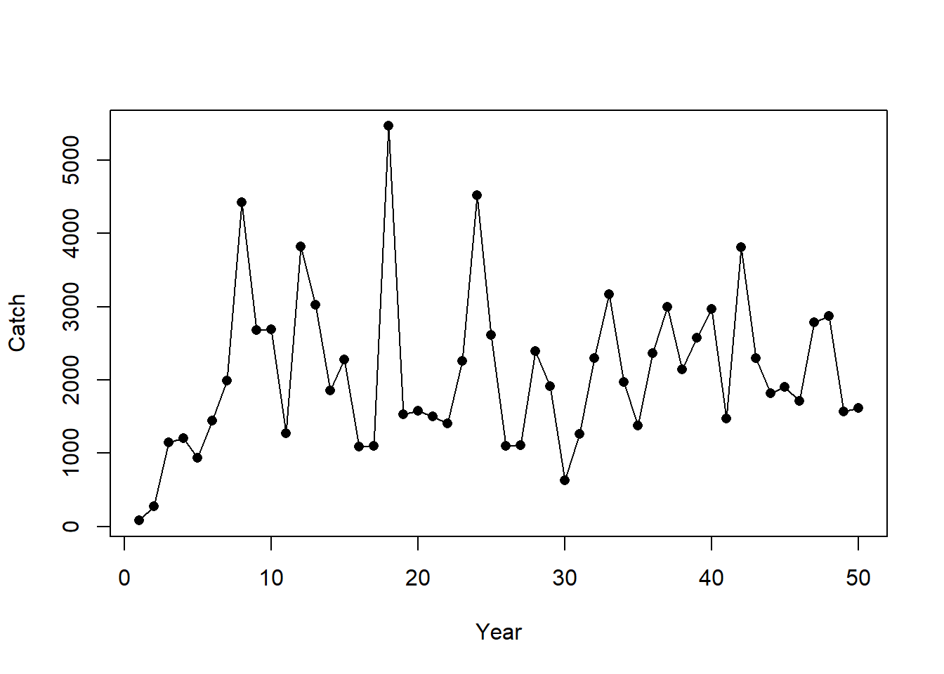
and by checking that the simulated catch multiplied by the catch observation error is the same as the real catch data provided in the OM:

plot(Data@Cat[1,], pch=16, xlab="Year", ylab="Catch")
lines(SimCatch * Hist@SampPars$Obs$Cobs_y[sim,1:OM@nyears])

Presented more generally in equations, catch observation error \(E^\text{obs}\) for simulation i in year y:

\[E^\text{obs}_{i,y} = E^\text{err}_{i,y} E^\text{bias}_i\] where \(E^\text{bias}_i\) is bias, calculated as the ratio of mean observed catch \(\bar{C^\text{obs}_i}\) to the mean simulated catch \(\bar{C^\text{sim}_i}\):

\[E^\text{bias}_i = \frac{\bar{C^\text{obs}_i}}{\bar{C^\text{sim}_i}}\] and \(E^\text{err}_{i,y}\) is the observation error calculated as:

\[E^\text{err}_{i,y} = \frac{C^\text{obs}_i}{(C^\text{sim}_i E^\text{bias}_i)}\]

Note that observation parameters that are related to Catch Sampling (e.g., OM@Cobs) are ignored when the OM is conditioned on catch data.

Generate Catch Observation Error for Projection Period

The statistical properties of the catch observation error, conditioned on the observed real catches as demonstrated above, are used to generate the catch observation error for the projection years.

Although all these calculations occur internally, we demonstrate the code here, again for simplicity just showing a single simulation (sim 2).

We calculate the standard deviation in log-space of the standardized catch observation error for the last 10 years of the historical period:

nyears <- OM@nyears
# standardized catch error to mean 1
Cerr.st <- Cerr[max(nyears-10, 1):nyears]/mean(Cerr[max(nyears-10, 1):nyears])

# standard deviation of log(Cerr.st)
Csd <- sd(log(Cerr.st))

And then generate log-normally distributed catch variability with this standard deviation for the projection years:

# Generate log-normal variability for projection years with same SD
Cerr_proj <- exp(rnorm(OM@proyears, -Csd^2/2, Csd))

Finally, we add the catch bias to the catch variability to produce the catch observation error for the projection period:

# add catch bias
Cobs_proj <- Cerr_proj * Cbias

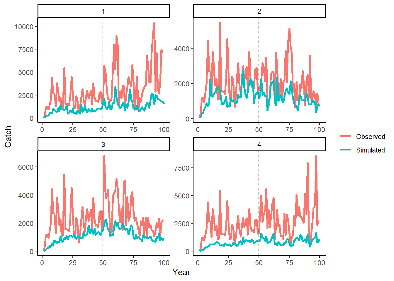
We can demonstrate that the simulated observed catches in the projection period maintain the same statistical properties as the catch observation error calculated from the historical period.

First, simulate the projection period with an example reference MP:

MSE <- Project(Hist, MPs="FMSYref", silent=TRUE)

Then we plot the simulated ‘observed’ data (i.e., data passed internally to the MPs) and ‘real’ catches (provided in OM for historical period) (note the last projection year of ‘observed’ data is not available and is replaced with NAs):

library(ggplot2)
library(tidyr)
library(dplyr)
DF <- data.frame(Sim=1:OM@nsim,
                 Year=rep(1:(OM@nyears+OM@proyears), each=OM@nsim),
                 Simulated=c(as.vector(MSE@CB_hist), as.vector(MSE@Catch[,1,])),
                 Observed=as.vector(cbind(MSE@PPD[[1]]@Cat, rep(NA, OM@nsim)))) %>% 
  tidyr::pivot_longer(cols=3:4) 

ggplot(DF, aes(x=Year, y=value, color=name)) +
  facet_wrap(~Sim, scales="free") +
  geom_line(size=1.2) +
  theme_classic() +
  geom_vline(xintercept = OM@nyears, linetype=2) + 
  labs(y="Catch", color="")

## Warning: Removed 1 row(s) containing missing values (geom_path).

These plots visually demonstrate that the statistical relationship between the simulated and observed catch data in the historical period (years 1–50) is maintained in the projection period (years 51–100).