Add Data to OM
To condition our OM with index data, we create a blank Data object:
Data <- new('Data')and populate the Year, Ind, and CV_Ind slots with our observed data:
# years - must be length(OM@nyears)
Data@Year <- RealData@Year

# 'real' index (can be patchy)
Data@Ind <- RealData@Ind[1,,drop=FALSE]

# assumed CV=0.2 all years
Data@CV_Ind <- matrix(0.2, nrow=1, ncol=length(Data@Year))
and add the Data object to the cpars slot:
OM@cpars$Data <- DataIn this example, we are using the index of total abundance (Data@Ind). The same process is followed to add a real spawning index (Data@SpInd) or vulnerable biomass index (Data@VInd) (or, if you’re feeling brave, all three at the same time!).
Condition Index Observation Model
The observation model is conditioned on the index data when the historical spool-up period is simulated:
Hist <- Simulate(OM, silent=TRUE)We can now compare our simulated index with our ‘real’ observed index:
# The index data that are passed to the MPs
ObsInd <- Hist@Data@Ind

# first 5 years of the 'real' index data
OM@cpars$Data@Ind[1,1:5]
## [1] 2.474687 3.161074 2.628440 2.215063 2.494472# first 5 years of simulated 'observed' index data passed to MPs
ObsInd[,1:5]## [,1] [,2] [,3] [,4] [,5]
## [1,] 2.474687 3.161074 2.62844 2.215063 2.494472
## [2,] 2.474687 3.161074 2.62844 2.215063 2.494472
## [3,] 2.474687 3.161074 2.62844 2.215063 2.494472
## [4,] 2.474687 3.161074 2.62844 2.215063 2.494472# first 5 years of index data simulated from OM
Biomass <- apply(Hist@TSdata$Biomass, 1:2, sum) # sum over areas
Index <- Biomass/apply(Biomass,1, mean)
Index[,1:5]## [,1] [,2] [,3] [,4] [,5]
## [1,] 1.5580913 1.3945556 1.577345 1.783264 1.226909
## [2,] 1.4965929 1.6967884 1.540443 1.394663 1.389259
## [3,] 0.9432994 0.8984943 1.002991 1.044759 1.095903
## [4,] 1.2517973 1.1888758 1.171071 1.190840 1.227618The index observation error Iobs_y in the observation model is updated based on the difference between the ‘real’ index data and the index data simulated from the OM. We demonstrate how the index observation error is calculated here for one simulation:
# simulated index from 1 simulation
sim <- 2
SimIndex <- Index[sim,1:OM@nyears]

# our 'real' index data
ObsIndex <- Data@Ind[1,]
Use the internal function indfit to calculate hyper-stability parameter beta, and autocorrelation and standard deviation in the log residuals:
ind.prop <- MSEtool:::indfit(SimIndex, ObsIndex, plot=T, Year=1:OM@nyears)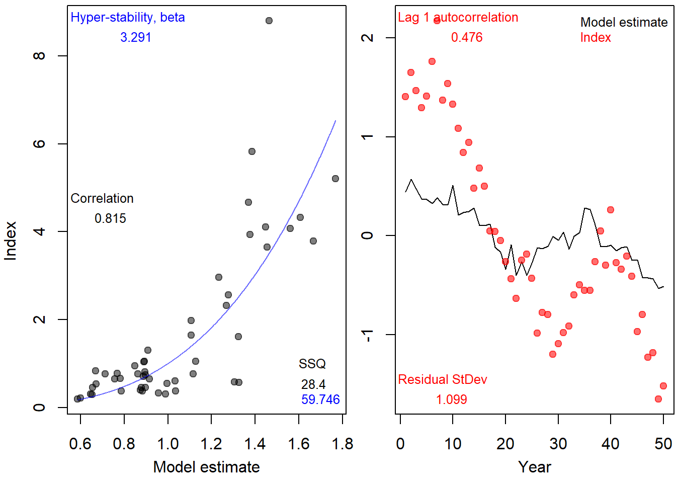
ind.prop## beta AC sd cor AC2 sd2
## 1 3.291333 0.4758299 0.6079967 0.8154966 0.873177 0.7613037And then calculate the observation error for the index in the historical years.
# internal function to log and standardise to mean 0
lcs <- MSEtool:::lcs

# Index observation error
Ierr_y <- exp(lcs(ObsIndex))/exp(lcs(SimIndex))^ind.prop$beta
You can confirm that the updated index observation error parameters match Ierr_y for simulation 2:
# check Obs$Iobs_y is the same
cbind(Ierr_y,Hist@SampPars$Obs$Ierr_y[sim,1:OM@nyears])
and by checking that the simulated standardized biomass multiplied by the index observation error is the same as the real index data provided in the OM:
plot(Data@Ind[1,], pch=16, xlab="Year", ylab="Index")
SimIndex <- exp(lcs(SimIndex))^ind.prop$beta* Hist@SampPars$Obs$Ierr_y[sim,1:OM@nyears]
SimIndex <- SimIndex/mean(SimIndex)
lines(SimIndex)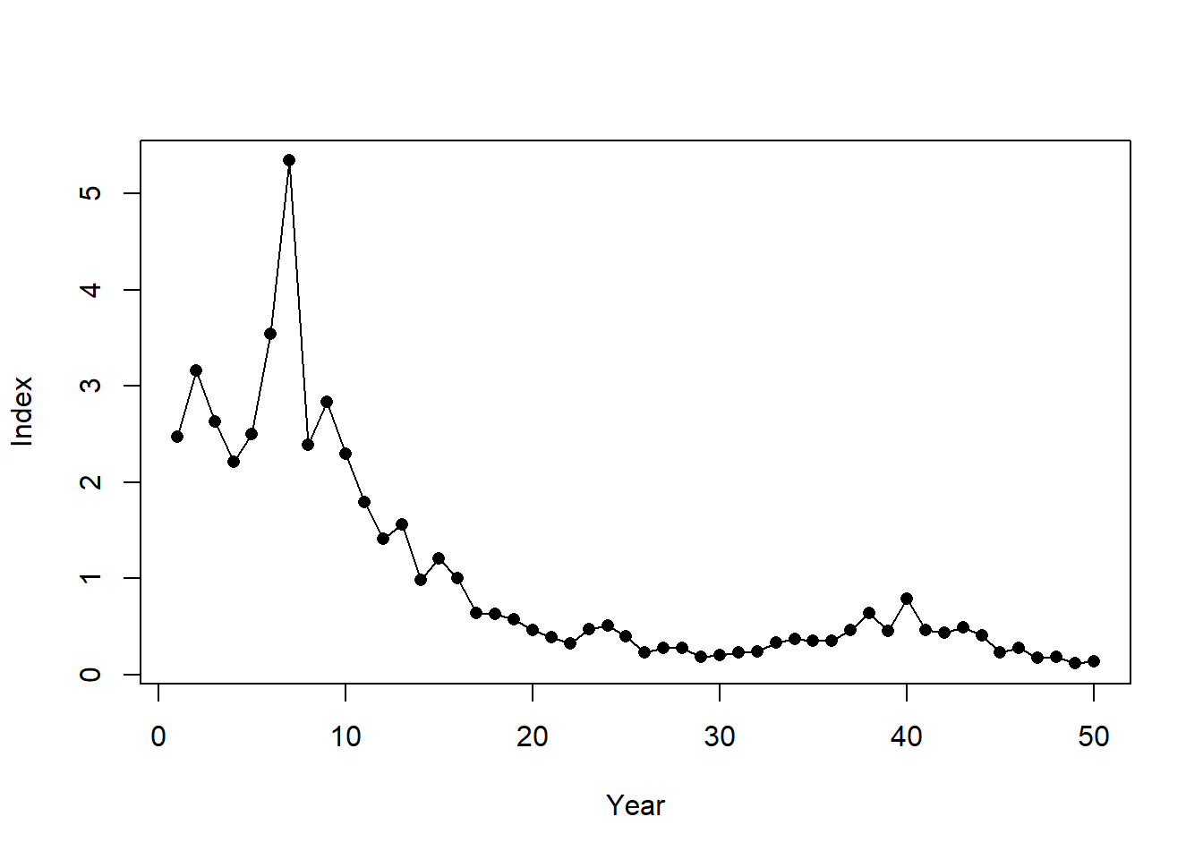
Note that observation parameters that are related to Index Sampling (e.g., OM@Iobs) are ignored when the OM is conditioned on index data.
Generate Index Observation Error for Projection Period
The statistical properties of the index observation error, conditioned on the observed real index as demonstrated above, are used to generate the index observation error for the projection years.
Although all these calculations occur internally, we demonstrate the code here, again for simplicity just showing a single simulation (sim 2).
We use the internal function generateRes to generate the residuals with the specified autocorrelation and standard deviation (in log space):
MSEtool:::generateRes## function(df, nsim, proyears, lst.err) {
## sd <- df$sd
## ac <- df$AC
## if (all(is.na(sd))) return(rep(NA, nsim))
## mu <- -0.5 * (sd)^2 * (1 - ac)/sqrt(1 - ac^2)
## Res <- matrix(rnorm(proyears*nsim, mu, sd), nrow=proyears, ncol=nsim, byrow=TRUE)
## # apply a pseudo AR1 autocorrelation
## Res <- sapply(1:nsim, applyAC, res=Res, ac=ac, max.years=proyears, lst.err=lst.err) # log-space
## exp(t(Res))
## }
## <bytecode: 0x000000002b7feb68>
## <environment: namespace:MSEtool>Ierr_proj <- MSEtool:::generateRes(ind.prop, nsim=1, proyears=50,
lst.err=log(Hist@SampPars$Obs$Ierr[sim,OM@nyears]))We can demonstrate that the simulated observed catches in the projection period maintain the same statistical properties as the catch observation error calculated from the historical period.
First, simulate the projection period with an example reference MP:
MSE <- Project(Hist, MPs="FMSYref", silent=TRUE)Then we plot the simulated ‘observed’ data (i.e., data passed internally to the MPs) and ‘real’ catches (provided in OM for historical period) (note the last projection year of ‘observed’ data is not available and is replaced with NAs):
library(ggplot2)
library(tidyr)
library(dplyr)

HistBiomass <- apply(Hist@TSdata$Biomass, 1:2, sum)
ProjBiomass <- MSE@B[,1,]
AllBiomass <- cbind(HistBiomass, ProjBiomass)

Simulated <- AllBiomass/apply(AllBiomass, 1, mean)
Observed <- cbind(MSE@PPD[[1]]@Ind, rep(NA, OM@nsim))
Observed <- Observed/apply(Observed, 1, mean, na.rm=TRUE)

DF <- data.frame(Sim=1:OM@nsim,
                 Year=rep(1:(OM@nyears+OM@proyears), each=OM@nsim),
                 Simulated=as.vector(Simulated),
                 Observed=as.vector(Observed)) %>%
  tidyr::pivot_longer(cols=3:4)

ggplot(DF, aes(x=Year, y=value, color=name)) +
  facet_wrap(~Sim, scales="free") +
  geom_line(size=1.2) +
  theme_classic() +
  geom_vline(xintercept = OM@nyears, linetype=2) +
  labs(y="Index", color="")
## Warning: Removed 1 row(s) containing missing values (geom_path).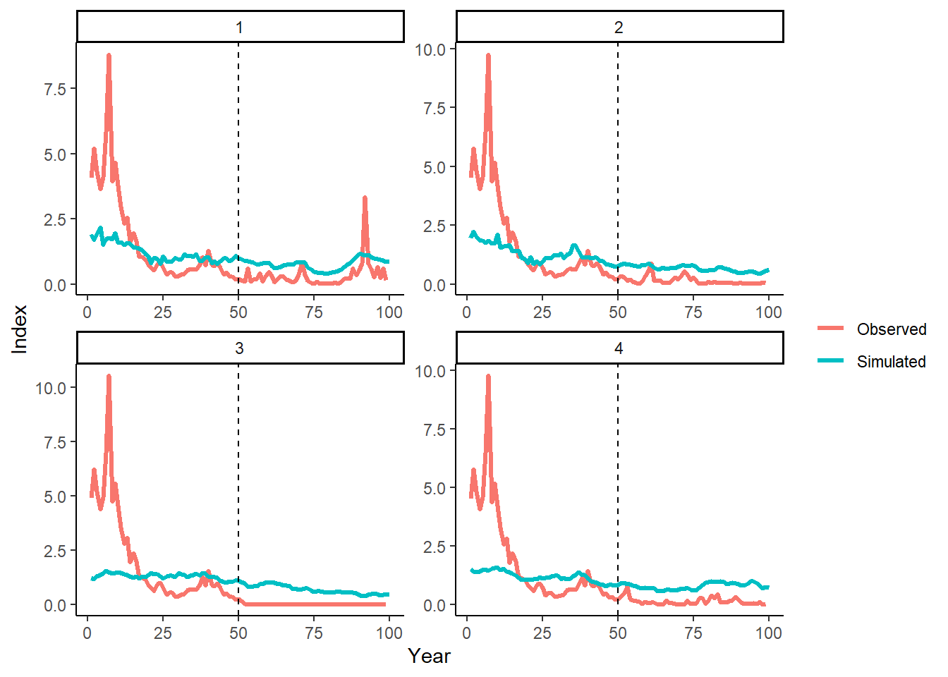
These plots visually demonstrate that the statistical relationship between the simulated and observed index data in the historical period (years 1–50) is maintained in the projection period (years 51–100).