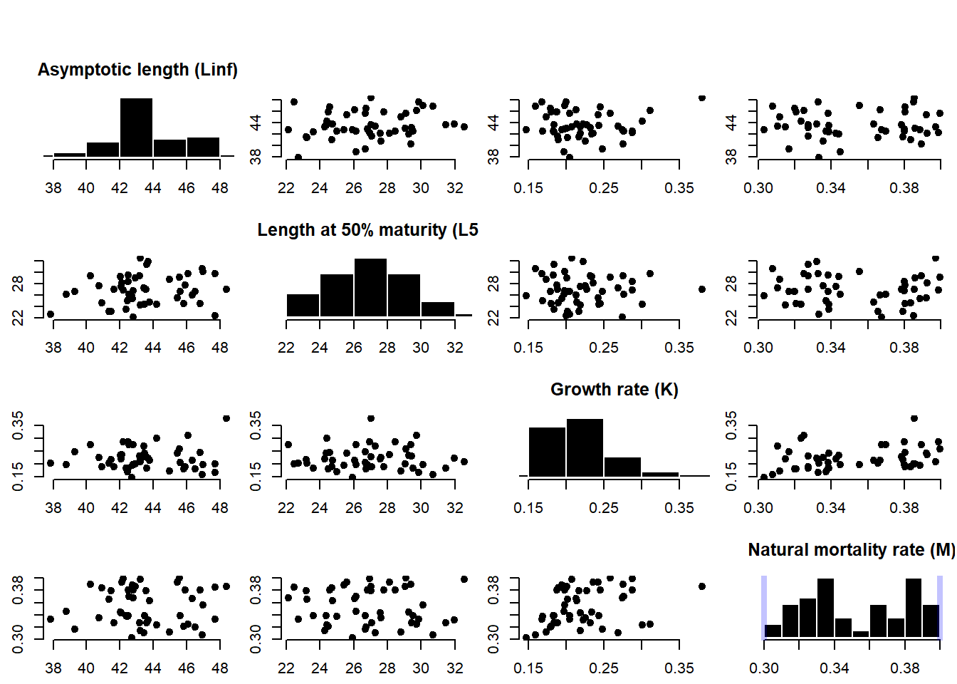
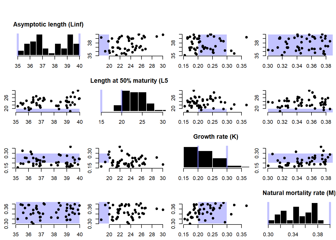
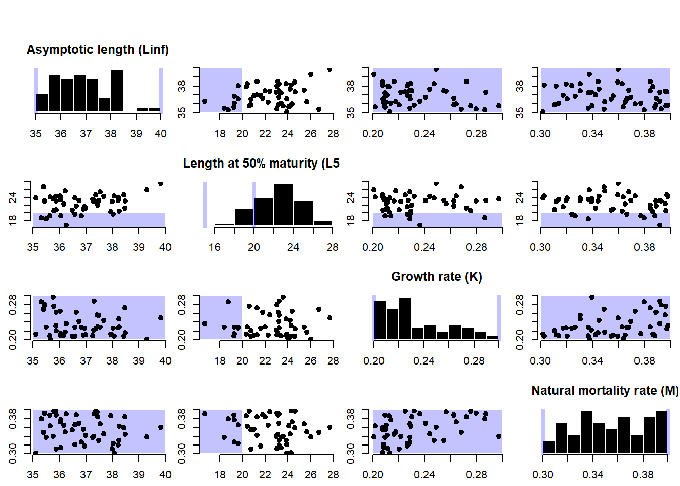
The LH2OM function can be used to force correlation between the life-history parameters, or predict values for missing life-history parameters.
Thorson et al. (2017) developed a hierarchical model, based on records available in FishBase, to predict life-history parameters for all 33,000+ fish species listed within FishBase. The LH2OM function uses the Thorson et al. (2017) model to generate correlated samples of the life-history parameters based on the relevant taxonomic information (Class, Family, Genus, and Species) for the species being modelled in the MSE.
The approach uses taxonomic information and any available information on the life-history parameters of the species in the OM to generate predictions of the missing parameters. For example, if no knowledge exists on the four life-history parameters (Linf, L50, M, and K), the model uses the taxonomic information (first Genus and Species, and if records don’t exist for this species in FishBase, then up a taxonomic level to Family, and so on) to generate predicted values for all four parameters. If information is available for some parameters, e.g., reasonable bounds on Linf and M for the species, the hierarchical model is used to generate predictions of the corresponding L50 and K values. That is, the observed ratios of L50/Linf and M/K are maintained. In this way the simulated life-history strategies are biologically realistic, and are appropriate for the species being modelled in the MSE.
Predicting all life-history parameters
The LH2OM function can be used to predict the four correlated life-history parameters (Linf, L50, M, and K) using only the available taxonomic information (only for fish species).
For example, here we create an empty OM object, populate the Species slot and use the LH2OM function to predict the life-history parameters using hierarchical model:
OM <- new("OM")
OM@Species <- "Scomber japonicus"
OM <- LH2OM(OM)
## Predicting Linf## Predicting L50## Predicting K## Predicting M## Species match: Actinopterygii Perciformes Scombridae Scomber japonicus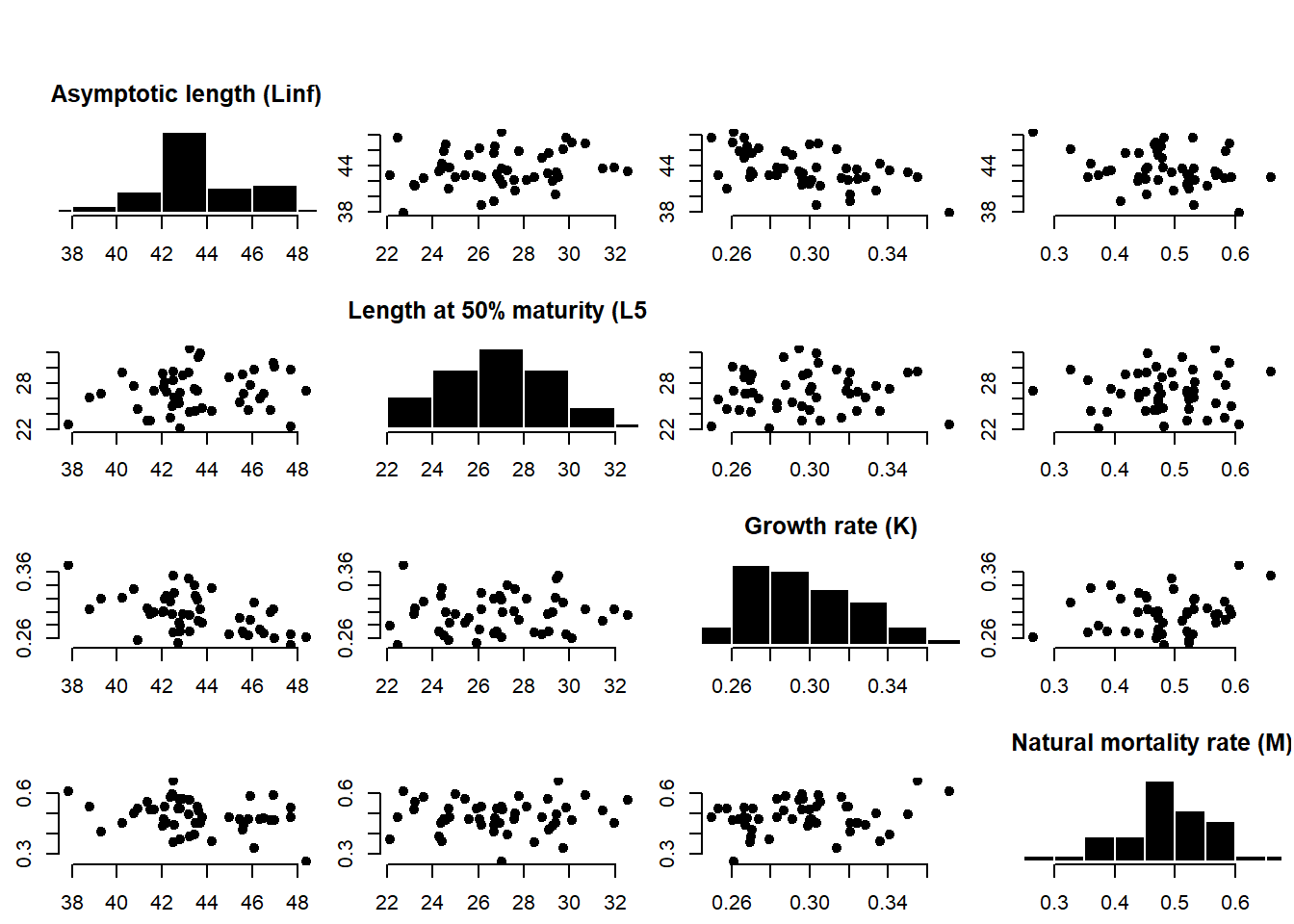
After using the LH2OM function, the cpars slot is populated with OM@nsim correlated samples of the life-history parameters:
str(OM@cpars)## List of 4
## $ Linf: num [1:48] 42.5 40.9 42.4 47.7 40.7 ...
## $ M : num [1:48] 0.357 0.523 0.582 0.483 0.498 ...
## $ K : num [1:48] 0.27 0.258 0.316 0.25 0.334 ...
## $ L50 : num [1:48] 28.5 24.7 23.6 22.5 27.6 ...Notice also that the OM@M slot is no longer used after the LH2OM function has been run on the OM object:
OM@M## [1] 0 0Predicting some life-history parameters
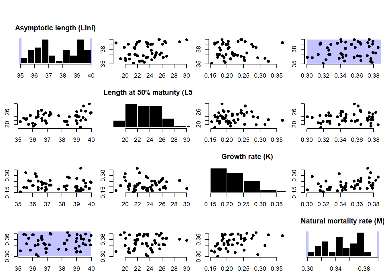
In some cases local estimates of life-history parameters may be available which are more reliable and less variable than those predicted from the FishBase database. For example, suppose that we had estimates of the natural mortality rate (M) for our stock that ranged between 0.3 and 0.4. We populate the OM@M slot with these values and use LH2OM to predict the correlated K parameter values:
OM <- new("OM")
OM@Species <- "Scomber japonicus"
OM@M <- c(0.3, 0.4)
OM <- LH2OM(OM)
## Predicting Linf## Predicting L50## Predicting K## Predicting K from M## Species match: Actinopterygii Perciformes Scombridae Scomber japonicus