In this section we dive into the contents of MP functions in more detail.
Let’s examine an existing output MP to identify the MP data requirements.
Since we’ve seen it used as a default MP in other examples, let’s learn more about how DCAC function in the DLMtool package. Type ?DCAC in the R console or visit the DCAC MP documentation page for details on the DCAC MP.
We can see the code for the DCAC MP by simply typing the name of the MP into the console (this is a fantastic advantage of using R - there is complete transparency about package functions):
DCAC## function (x, Data, reps = 100, plot = FALSE)
## {
## rundcac <- DCAC_(x, Data, reps, updateD = TRUE)
## TAC <- MSEtool::TACfilter(rundcac$dcac)
## if (plot)
## DCAC_plot(x, Data, dcac = rundcac$dcac, TAC, Bt_K = rundcac$Bt_K,
## yrs = 1:length(Data@Year))
## Rec <- new("Rec")
## Rec@TAC <- TAC
## Rec
## }
## <bytecode: 0x000000001a577b48>
## <environment: namespace:DLMtool>
## attr(,"class")
## [1] "MP"There are several versions of the DCAC MP in the DLMtool package (this version updates the estimated depletion in the projection period). We can see that DCAC is a wrapper for the internal DCAC_ function.
Let’s print out the contents of the DCAC_ function:
DCAC_## function (x, Data, reps = 100, Bt_K = NULL, updateD = FALSE)
## {
## if (length(Data@Year) < 1)
## return(list(dcac = NA, Bt_K = NA, BMSY_K = NA))
## if (MSEtool::NAor0(Data@BMSY_B0[x]))
## stop("Data@BMSY_B0 is NA")
## if (MSEtool::NAor0(Data@CV_BMSY_B0[x]))
## stop("Data@CV_BMSY_B0 is NA")
## yr.lst <- match(Data@LHYear[1], Data@Year)
## yrs <- 1:yr.lst
## C_tot <- Data@AvC[x] * Data@t[x]
## Mdb <- MSEtool::trlnorm(reps, Data@Mort[x], Data@CV_Mort[x])
## FMSY_M <- MSEtool::trlnorm(reps, Data@FMSY_M[x], Data@CV_FMSY_M[x])
## if (is.null(Bt_K))
## Bt_K <- MSEtool::trlnorm(reps, Data@Dt[x], Data@CV_Dt[x])
## if (!updateD) {
## if (Data@LHYear[1] != max(Data@Year)) {
## dcac <- rep(Data@MPrec[x], reps)
## return(list(dcac = dcac, Bt_K = Bt_K))
## }
## }
## Bt_K[Bt_K > 1] <- 1
## Bt_K[Bt_K < 0] <- 0
## if (any(is.na(c(Data@BMSY_B0[x], Data@CV_BMSY_B0[x])))) {
## warning("Data@BMSY_B0 or Data@CV_BMSY_B0 do not contain values")
## return(list(dcac = rep(NA, reps), Bt_K = Bt_K))
## }
## BMSY_K <- rbeta(reps, MSEtool::alphaconv(Data@BMSY_B0[x],
## Data@BMSY_B0[x] * Data@CV_BMSY_B0[x]), MSEtool::betaconv(Data@BMSY_B0[x],
## Data@BMSY_B0[x] * Data@CV_BMSY_B0[x]))
## dcac <- C_tot/(yr.lst + ((1 - Bt_K)/(BMSY_K * FMSY_M * Mdb)))
## return(list(dcac = dcac, Bt_K = Bt_K, BMSY_K = BMSY_K))
## }
## <bytecode: 0x0000000019609708>
## <environment: namespace:DLMtool>“Crikey that looks complicated!” might be your first reaction. However this output MP function is easily demystified.
Like all MPs it has four main arguments: x, Data, reps and plot (the last argument is optional), plus, because this function is accessed via a wrapper, a few that are specific to this MP.
The argument x is the position in the Data object. When real data are stored in a Data object, there is only one position - there is only one real data set.
However, in MSE we conduct many simulations and x refers to simulated data from simulation number x. Any single parameters such as natural mortality rate (Mort) are a vector (nsim long). See Data@Mort[x] in the DCAC code. Any time series such as annual catches or relative abundance indices, are a matrix of nsim rows and nyears columns.
A range of example objects of class Data are available:
avail('Data')## Searching for objects of class Data in package: MSEtool## Searching for objects of class Data in package: SAMtool## Searching for objects of class Data in package: DLMtool## [1] "Atlantic_mackerel" "China_rockfish" "Cobia"
## [4] "Example_datafile" "Gulf_blue_tilefish" "ourReefFish"
## [7] "Red_snapper" "SimulatedData" "Simulation_1"
## [10] "swordfish"For simplicity lets use a Data object with just two simulations, SimulatedData and rename it Data
Data <- SimulatedDataSince there are only three simulations in this data set (3 positions) we can now see three values of natural mortality rate:
Data@Mort## [1] 0.3657912 0.4662769 0.4147479And a matrix of catches with three rows:
Data@Cat## [,1] [,2] [,3] [,4] [,5] [,6] [,7]
## [1,] 82.33424 272.3924 1151.6952 1209.5023 938.6177 1447.9005 1986.240
## [2,] 37.74578 227.4069 918.9217 756.4462 1361.4852 409.7910 1257.849
## [3,] 47.64502 111.2415 436.3407 646.7710 1074.2779 543.5588 451.440
## [,8] [,9] [,10] [,11] [,12] [,13] [,14]
## [1,] 4424.6721 2680.7514 2687.3781 1275.759 3822.4663 3025.4098 1860.4249
## [2,] 733.6195 1536.2300 2200.2678 2053.099 2993.6751 1740.6164 2911.5760
## [3,] 546.2285 617.3952 668.4834 1092.319 983.5743 699.7499 617.4867
## [,15] [,16] [,17] [,18] [,19] [,20] [,21]
## [1,] 2279.2725 1090.3048 1103.5952 5462.8762 1534.1317 1575.4004 1501.754
## [2,] 1680.0477 1514.0509 2716.8478 1707.7156 1520.2907 1961.8084 2025.587
## [3,] 376.2699 295.4171 940.0009 524.6327 810.2256 748.9694 1063.138
## [,22] [,23] [,24] [,25] [,26] [,27] [,28]
## [1,] 1405.3164 2256.311 4519.724 2611.2848 1100.1405 1106.2004 2388.5010
## [2,] 1979.3770 1436.991 1837.329 1499.3278 1365.0436 2350.2626 2774.1018
## [3,] 786.0475 1421.989 1093.460 550.2417 795.2361 411.7311 599.3514
## [,29] [,30] [,31] [,32] [,33] [,34] [,35]
## [1,] 1915.2016 634.5498 1265.481 2295.5705 3168.9819 1973.3079 1375.005
## [2,] 1064.4816 1395.5550 1581.387 2283.1141 2704.0911 1039.0900 1022.632
## [3,] 534.8014 891.3572 1564.871 251.2743 417.6512 977.8942 1073.009
## [,36] [,37] [,38] [,39] [,40] [,41] [,42]
## [1,] 2367.5795 2998.8700 2145.9105 2571.2752 2970.2587 1471.5750 3813.0373
## [2,] 1470.2503 1271.3841 1461.0880 1158.7410 709.8860 1579.0602 1368.2224
## [3,] 281.1288 675.7261 471.1569 720.5783 358.3763 745.1902 479.4397
## [,43] [,44] [,45] [,46] [,47] [,48] [,49]
## [1,] 2292.1426 1819.199 1902.6963 1717.1045 2788.4449 2873.1566 1567.1967
## [2,] 1741.4837 1556.353 1106.7210 1924.2976 1202.6243 1828.9854 1457.3277
## [3,] 998.9998 1076.016 752.0612 756.1286 327.0441 687.9081 285.3886
## [,50]
## [1,] 1614.543
## [2,] 2037.379
## [3,] 398.655We could generate a single TAC recommendation from these data using DCAC by specifying position 1 (for the first simulation) and by setting reps=1 (we want a single DCAC TAC recommendation)
DCAC(x=1,Data,reps=1)## TAC (median)
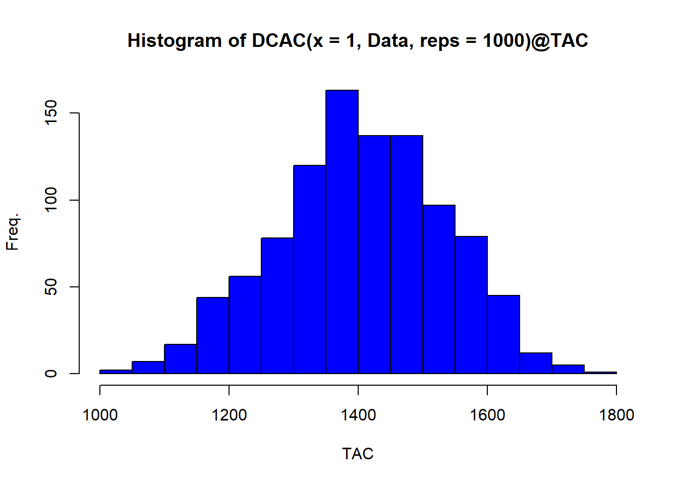
## 1411.557If we wanted a stochastic estimate of the TAC we could increase the number of reps:
hist(DCAC(x=1,Data,reps=1000)@TAC,xlab="TAC",ylab="Freq.",col="blue")
In the next section we describe how to build custom MPs.