openMSE was designed to be extensible in order to promote the development of new Management Procedures. In this section we design a series of new Management Procedures that include spatial controls and input controls in the form of size limit restrictions.
If you wish, you can also add your newly developed MPs to the package so they are accessible to other uses. Of course you will be credited as the author. Please contact us for details how to do this.
As described in the Populating the Data object section, real data are stored in a class of objects Data.
The runMSE function generates simulated data and puts it in exactly the same format as real data. This is highly desirable because
it means that the same MP code that is tested in the MSE can then be used to make management recommendations.
If an MP is coded incorrectly it may catastrophically fail MSE testing and will therefore be excluded from use in management.
A Constant Catch MP
We’ve now got a better idea of the anatomy of an MP. It is a function that must accept three arguments (we will ignore plot for now):
- x: a simulation number
- Data: an object of class
Data - reps: the MP can provide a sample of TACs
repslong.
Let’s have a go at designing our own custom MP that can work with openMSE We’re going to develop an MP that sets the TAC as the ‘3rd highest catch’.
We decide to call our function THC
THC<-function(x, Data, reps){

  # Find the position of third highest catch

  THCpos<-order(Data@Cat[x,],decreasing=T)[3]

  # Make this the mean TAC recommendation

  THCmu<-Data@Cat[x,THCpos]

  # A sample of the THC is taken according to a fixed CV of 10%
  TACs <- THCmu * exp(rnorm(reps, -0.1^2/2, 0.1)) # this is a lognormal distribution

  Rec <- new("Rec") # create a 'Rec'object
  Rec@TAC <- TACs # assign the TACs to the TAC slot
  Rec # return the Rec object
}
To recap that’s just seven lines of code:
THC<-function(x, Data, reps){
  THCpos<-order(Data@Cat[x,],decreasing=T)[3]
  THCmu<-Data@Cat[x,THCpos]
  Rec <- new("Rec")
  Rec@TAC <- THCmu * exp(rnorm(reps, -0.1^2/2, 0.1))
  Rec
}
We can quickly test our new MP for the example Data object
THC(x=1,Data,reps=10)@TAC## [1] 4084.666 4233.960 4320.225 4247.745 3975.688 4635.546 4017.359 4417.738
## [9] 4813.774 5363.664Now that we know it works, to make the function compatible with the DLMtool package we have to assign it the class ‘MP’ so that DLMtool recognizes the function as a management procedure
class(THC)<-"MP"A More Complex MP
The THC MP is simple and frankly not a great performer (depending on depletion, life-history, adherence to TAC recommendations).
Let’s innovate and create a brand new MP that could suit a catch-data-only stock like Indian Ocean Longtail tuna!
It may be possible to choose a single fleet and establish a catch rate that is ‘reasonable’ or ‘fairly productive’ relative to current catch rates. This could be for example, 40% of the highest catch rate observed for this fleet or, for example, 150% of current cpue levels.
It is straightforward to design an MP that will aim for this target index level by making adjustments to the TAC.
We will call this MP TCPUE, short for target catch per unit effort:
TCPUE<-function(x,Data,reps=100){

  mc<-0.05                             # max change in TAC
  frac<-0.3                            # target index is 30% of max
  nyears<-length(Data@Ind[x,])         # number of years of data

  smoothI<-smooth.spline(Data@Ind[x,]) # smoothed index
  targetI<-max(smoothI$y)*frac         # target

  currentI<-mean(Data@Ind[x,(nyears-2):nyears]) # current index

  ratio<-currentI/targetI              # ratio currentI/targetI

  if(ratio < (1 - mc)) ratio <- 1 - mc # if currentI < targetI
  if(ratio > (1 + mc)) ratio <- 1 + mc # if currentI > targetI

  Rec <- new("Rec")
  Rec@TAC <- Data@MPrec[x] * ratio * exp(rnorm(reps, -Data@CV_Ind[x]^2/2, Data@CV_Ind[x]))
  Rec
}
The TCPUE function simply decreases the past TAC (stored in Data@MPrec) if the index is lower than the target and increases the TAC if the index is higher than the target.
All that is left is to assign the function as class MP so that openMSE recognizes it as a management procedure:
class(TCPUE)<-"MP"Beyond the Catch Limit
All management procedures return an object of class Rec that contains 13 slots:
slotNames("Rec")## [1] "TAC" "Effort" "Spatial" "Allocate" "LR5" "LFR"
## [7] "HS" "Rmaxlen" "L5" "LFS" "Vmaxlen" "Fdisc"
## [13] "DR" "Misc"We’ve already seen the TAC slot in the previous example. The remaining slots relate to various forms of input control:
- Effort (total allowable effort (TAE) relative to last historical year)
- Spatial - Fraction of each area that is open
- Allocate - Allocation of effort from closed areas to open areas
- LR5 - Length at 5% retention
- LFR - Length at 100% retention
- HS - Upper slot limit
- Rmaxlen - Retention of the maximum length class
- L5 - Length at 5% selection (e.g a change in gear type)
- LFS - Length at 100% selection (e.g a change in gear type)
- Vmaxlen - Selectivity of the maximum length class
- Fdisc - Update the discard mortality if required
- Misc - An optional slot for storing additional information
See the help documentation or type class?Rec in the R console for more information on the contents of the Rec object.
The curE MP just keeps effort constant at current levels:
curE## function (x, Data, reps, plot = FALSE)
## {
## rec <- new("Rec")
## rec@Effort <- 1
## if (plot)
## curE_plot(x, rec, Data)
## rec
## }
## <bytecode: 0x000000001d76bf68>
## <environment: namespace:DLMtool>
## attr(,"class")
## [1] "MP"Note that only the Effort slot in the Rec object is populated in this case.
To highlight the differences among Input control MPs, examine the spatial control MP MRreal that closes area 1 to fishing and reallocates fishing to the open area 2:
MRreal## function (x, Data, reps, plot = FALSE)
## {
## rec <- new("Rec")
## rec@Allocate <- 1
## rec@Spatial <- c(0, rep(1, Data@nareas - 1))
## if (plot)
## barplot(rec@Spatial, xlab = "Area", ylab = "Fraction Open",
## ylim = c(0, 1), names = 1:Data@nareas)
## return(rec)
## }
## <bytecode: 0x000000001d8e1fc8>
## <environment: namespace:DLMtool>
## attr(,"class")
## [1] "MP"In contrast MRnoreal does not reallocate fishing effort:
MRnoreal## function (x, Data, reps, plot = FALSE)
## {
## rec <- new("Rec")
## rec@Allocate <- 0
## rec@Spatial <- c(0, rep(1, Data@nareas - 1))
## if (plot)
## barplot(rec@Spatial, xlab = "Area", ylab = "Fraction Open",
## ylim = c(0, 1), names = 1:Data@nareas)
## return(rec)
## }
## <bytecode: 0x000000001da75a08>
## <environment: namespace:DLMtool>
## attr(,"class")
## [1] "MP"The MP matlenlim only specifies the parameters of length retention using an estimate of length at 50% maturity (Stock@L50):
matlenlim## function (x, Data, reps, plot = FALSE)
## {
## rec <- new("Rec")
## rec@LFR <- Data@L50[x]
## rec@LR5 <- rec@LFR * 0.95
## if (plot)
## size_lim_plot(x, Data, rec)
## rec
## }
## <bytecode: 0x000000001dd82db0>
## <environment: namespace:DLMtool>
## attr(,"class")
## [1] "MP"An Example Effort Control
Here we will copy and modify the MP we developed earlier to specify a new version of the target catch per unit effort MP (TCPUE) that provides effort recommendations:
TCPUE_e<-function(x,Data,reps=100){

  mc<-0.05                             # max change in TAC
  frac<-0.3                            # target index is 30% of max
  nyears<-length(Data@Ind[x,])         # number of years of data

  smoothI<-smooth.spline(Data@Ind[x,]) # smoothed index
  targetI<-max(smoothI$y)*frac         # target

  currentI<-mean(Data@Ind[x,(nyears-2):nyears]) # current index

  ratio<-currentI/targetI              # ratio currentI/targetI

  if(ratio < (1 - mc)) ratio <- 1 - mc # if currentI < targetI
  if(ratio > (1 + mc)) ratio <- 1 + mc # if currentI > targetI

  rec <- new("Rec")
  rec@Effort <- Data@MPeff[x] * ratio
  rec

}
There have been surprisingly few changes to make TCPUE an input control MP that sets total allowable effort.
- We have had to use stored recommendations of effort in the
Data@MPeffslot, and - The final line of the MP is our input control recommendation that only modified the Effort.
That is all.
Again, we need to assign our new function to class MP:
class(TCPUE_e)<-"MP"Let’s test the two MPs and see how they [perform](/welcome-a-quick-tour/examining-results/:
testMSE<-runMSE(testOM,MPs=c("TCPUE","TCPUE_e"))## Checking MPs## Loading operating model## Optimizing for user-specified movement## Optimizing for user-specified depletion in last historical year## Calculating historical stock and fishing dynamics## Calculating MSY reference points for each year## Calculating B-low reference points## Calculating reference yield - best fixed F strategy## Simulating observed data## Running forward projections## 1 / 2 Running MSE for TCPUE## ..................................................## 2 / 2 Running MSE for TCPUE_e## ..................................................NOAA_plot(testMSE)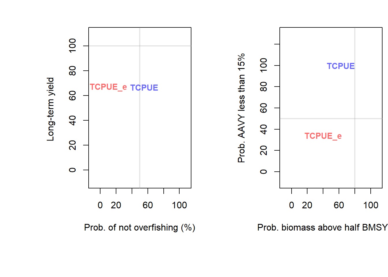
##         PNOF B50  LTY    VY
## TCPUE   55.3  62 66.7 100.0
## TCPUE_e 10.0  40 66.7  33.3