Sub-Sections
The MOM Object
The MOM object is not terribly different from a standard OM object.
slotNames('MOM')## [1] "Name" "Agency" "Region" "Sponsor" "Latitude"
## [6] "Longitude" "nsim" "proyears" "interval" "pstar"
## [11] "maxF" "reps" "cpars" "seed" "Source"
## [16] "Stocks" "Fleets" "Obs" "Imps" "CatchFrac"
## [21] "Allocation" "Efactor" "Complexes" "SexPars" "Rel"The big difference between objects of class OM and those of class MOM is that instead of including a slot for each parameter of the stock (Stock), fleet (Fleet), observation (Obs) and implementation (Imp) models for OM objects, MOM objects include these in four slots that are lists of entire Stock, Fleet, Obs and Imp objects - after all it’s multi-fleet and/or multi stock, right?!
Stocks, Fleets, Obs, and Imps
There are four new slots in an MOM object (compared to an OM object): MOM@Stocks, MOM@Fleets, MOM@Obs, and MOM@Imps.
MOM@Stocksis a list of stock objects (nstocks long)MOM@Fleetsis a hierarchical list of fleet objects (nstocks with fleets nested in stocks)MOM@Obsis a hierarchical list of observation error objects (nstocks with fleets nested in stocks)MOM@Impsis a hierarchical list of implementation error objects (nstocks with fleets nested in stocks)
Ideally you’d get your various dynamics from conditioned operating models either using the Rapid Conditioning Model
or using the various openMSE helper functions that read in stock assessment output. However, for simplicity we’ll demonstrate how to do multiMSE with some pre-existing Stock, Fleet, Obs, and Imp objects that are included in openMSE:
avail('Stock')## ✔ Searching for objects of class Stock in package: MSEtool## [1] "Albacore" "Blue_shark" "Bluefin_tuna"
## [4] "Bluefin_tuna_WAtl" "Butterfish" "Herring"
## [7] "Mackerel" "Porgy" "Rockfish"
## [10] "Snapper" "Sole" "Toothfish"avail('Fleet')## ✔ Searching for objects of class Fleet in package: MSEtool## [1] "DecE_Dom" "DecE_HDom" "DecE_NDom"
## [4] "FlatE_Dom" "FlatE_HDom" "FlatE_NDom"
## [7] "Generic_DecE" "Generic_FlatE" "Generic_Fleet"
## [10] "Generic_IncE" "IncE_HDom" "IncE_NDom"
## [13] "Low_Effort_Non_Target" "Target_All_Fish" "Targeting_Small_Fish"avail('Obs')## ✔ Searching for objects of class Obs in package: MSEtool## [1] "Generic_Obs" "Imprecise_Biased" "Imprecise_Unbiased"
## [4] "Perfect_Info" "Precise_Biased" "Precise_Unbiased"avail('Imp')## ✔ Searching for objects of class Imp in package: MSEtool## [1] "Overages" "Perfect_Imp"Let’s imagine that we lose our minds and decide to create a model that simulates interactions between bluefin tuna and herring (we think bluefin eat herring). We also want to simulate three fleets, a bluefin fleet, a herring fleet and a mixed fleet that somehow, against all the odds catches both bluefin and herring! About as hypothetical as it gets I know, but that is intentional - this is just a demonstration!
First, we start off by creating the list of stock objects, this is pretty easy:
#                 Stock 1    Stock 2
Stocks <- list(Bluefin_tuna, Herring)
A key constraint here is that the Stock objects have the same number of areas (e.g. Bluefin_tuna@nareas).
We now want to create our fleets for these stocks. Our bluefin-only fleet has stable effort (premade fleet type Generic_FlatE) our herring-only fleet has increasing effort (premade fleet type Generic_IncE) and our mythical mixed fishery has decreasing effort (premade fleet type Generic_DecE).
This is the tricky bit.
Nominally, the same fleet occupies the same position for each stock. For example, ‘longline’ is fleet 1 for both bluefin and herring. However, the fleet interactions with the stocks can (and often will) be different - e.g. the trend in exploitation rate of the longline fleet may be stable for bluefin but decreasing for herring (in this admittedly bizarre case). That is why multiMSE requires the same number of fleets for each stock but you have to be able to specify unique fleet dynamics for each stock x fleet. For example longline_stable_exploitation could be Fleet 1 for bluefin and longline_decreasing_exploitation could be Fleet 1 for Herring - it is the same fleet but interacts differently with the two stocks.
A rare exception is if you have one fleet catching each stock. Then you can just have one fleet position for each stock and put the stock-specific fleet in position Fleet 1 for all stocks. Confused? I don’t blame you! But this should get clearer as you work through this guide.
To specify exploitation dynamics across stocks and fleets you create a hierarchical list structure (Fleets nested in Stocks):
#                           Fleet 1         Fleet 2      Fleet 3
Fleets_both_Stocks <- list(Generic_FlatE, Generic_IncE, Generic_DecE)
Fleets <- list( Fleets_both_Stocks, # Bluefin (position 1 in Stocks)
                Fleets_both_Stocks) # Herring (position 2 in Stocks)
# for the sake of this exercise we assume identical fleet dynamics for both stocks
Since each of these Fleets is going to generate fishery data for each stock, they each need an observation model by stock and fleet. Just like the Fleets list, this is hierarchical - Fleets nested in Stocks. We are going to assume that we get good data (Precise and Unbiased) for bluefin and bad data (Imprecise and Biased) for herring.
#                      Fleet 1             Fleet 2          Fleet 3
Bluefin_obs <- list(Precise_Unbiased, Precise_Unbiased, Precise_Unbiased)
Herring_obs <- list(Imprecise_Biased, Imprecise_Biased, Imprecise_Biased)
Obs <- list(Bluefin_obs,    # Bluefin (position 1 in Stocks)
             Herring_obs)    # Herring (position 2 in Stocks)
Lastly, we need to specify implementation error models for these, we are going to assume this is the same for both stocks and is fleet specific: perfect for the first 2 fleets and includes overages for the mixed fleet (fleet 3).
#                        Fleet 1       Fleet 2     Fleet 3
Imp_both_Stocks <- list(Perfect_Imp, Perfect_Imp, Overages)
Imps <- list( Imp_both_Stocks,   # Bluefin (position 1 in Stocks)
              Imp_both_Stocks)   # Herring (position 2 in Stocks)
Each of the stocks already has a prespecified range of depletion:
Bluefin_tuna@D## [1] 0.02 0.20Herring@D## [1] 0.05 1.00But how do we attribute the magnitude of historical exploitation among the various fleets?
Catch fractions by fleet for each stock
To allow multiMSE to run we need an extra Thing 1, and should have an additional Thing 2 after that.
Thing 1 is the current (most recent year) catch fractions among fleets for each stock. This information is required to calculate the relative catchabilities among the fleets.
Catch fractions are a list (nstock long) of matrices. Suppose we want 80% of current bluefin catches to come from fleet 1, 1% from fleet 2 and 19% from fleet 3, and also 60% of herring catches to come from Fleet 2, 5% from fleet 1 and the remaining 35% of herring catches from Fleet 3, this is how you would specify that:
nsim = 4
#                  Fleet1  Fleet2   Fleet3
bluefin_catchfrac<-c(0.8,   0.01,   0.19)
herring_catchfrac<-c(0.05,  0.6,    0.35)
CatchFrac <- list(
                  matrix( rep(bluefin_catchfrac, each=nsim), nrow=nsim),
                  matrix( rep(herring_catchfrac, each=nsim), nrow=nsim)
)

CatchFrac[[1]]
## [,1] [,2] [,3]
## [1,] 0.8 0.01 0.19
## [2,] 0.8 0.01 0.19
## [3,] 0.8 0.01 0.19
## [4,] 0.8 0.01 0.19The observant types among you will have noticed that we now need to specify the number of MSE simulations we are going to be doing (nsim). For now this is just 12 for demonstration purposes, but ultimately this would be >148 for a real MSE.
The reason we have done this is to allow for uncertainty in the catch fractions - the user could make catch fractions vary among fleets by simulation. For now, these are the same among simulations, which is the simplest thing, albeit a bit boring.
Specifying inter-stock relationships
You’ll remember that we said there was a Thing 2 that we should add to our multi-operating model. Ask yourself why we are modelling bluefin and herring together?
Because we want to look at an interaction between these stocks. If we didn’t, we would just model these stocks individually, and there would be only one stock in the Stocks slot and only one list of fleets in the Fleets slot (the remaining reason for modelling many stock without interactions is if they are managed by a single MP as a stock complex - we’ll come to this in a bit).
If we didn’t expect to set fleet-specific advice AND we weren’t modelling bluefin and herring interactions, we should just be using the regular runMSE and calculate the aggregate fleet dynamics (aggregate size vulnerability and trend in apical fishing mortality rate, for example).
But we’re demonstrating multiMSE here, and are therefore going to specify at least one relationship between the stocks (noting that you may wish to evaluate MPs that provide advice for a stock complex of multiple stock objects with no interactions - more below). The slot MOM@Rel is where you put these relationships as a list of R models with quite specific formatting.
Since we think bluefin are predators of herring, we are going to propose a relationship between bluefin abundance and the natural mortality rate of herring. Normally we would have derived this relationship empirically from data (in this case perhaps herring tagging survival estimates regressed on bluefin abundance estimates from a stock assessment).
However for the purposes of this demonstration we’re just going to cook something up out of thin air: nominally we are going to assume that herring have a natural mortality rate of 0.2 when there are no bluefin, and 0.4 when bluefin tuna are at unfished levels. To invent this relationship we are going to need to calculate bluefin unfished biomass from the operating model, make some fake data and fit an R model.
Here goes:
ages <- 1:60
bf_M <- mean(Bluefin_tuna@M)          # natural mortality rate
bf_Linf <- mean(Bluefin_tuna@Linf)    # asymptotic length
bf_K <- mean(Bluefin_tuna@K)          # von Bertalanffy growth parameter K
bf_t0 <- mean(Bluefin_tuna@t0)        # von B. theoretical age at length zero
bf_R0 <- Bluefin_tuna@R0              # unfished recruitment

bf_surv <- bf_R0*exp(-bf_M*(ages-1))             # survival
bf_wt_age <- bf_Linf*(1-exp(-bf_K*(ages-bf_t0))) # weight at age
bf_unfished <- sum(bf_R0*bf_surv*bf_wt_age)      # approxiate estimate of unfished biomass

M_err <- rlnorm(100,0,0.05)
M_2 <- seq(0.2,0.4,length.out=100) * M_err  # made up herring (stock 2) M values
B_1 <- seq(0,bf_unfished,length.out=100)    # made up bluefin tuna abundance levels

dat <- data.frame(M_2,B_1)
bfB_hM <- lm(M_2~B_1,dat=dat) # a linear model predicting M for stock 2 from biomass B for stock 1
summary(bfB_hM)
##
## Call:
## lm(formula = M_2 ~ B_1, data = dat)
##
## Residuals:
## Min 1Q Median 3Q Max
## -0.035640 -0.009224 0.000304 0.008397 0.033687
##
## Coefficients:
## Estimate Std. Error t value Pr(>|t|)
## (Intercept) 1.942e-01 2.786e-03 69.72 <2e-16 ***
## B_1 3.722e-10 8.811e-12 42.25 <2e-16 ***
## ---
## Signif. codes: 0 '***' 0.001 '**' 0.01 '*' 0.05 '.' 0.1 ' ' 1
##
## Residual standard error: 0.01403 on 98 degrees of freedom
## Multiple R-squared: 0.9479, Adjusted R-squared: 0.9474
## F-statistic: 1785 on 1 and 98 DF, p-value: < 2.2e-16Rel <- list(bfB_hM)plot(dat$B_1, dat$M_2,pch=19, xlab = "Bluefin biomass", ylab = "Herring natural mortality")
lines(dat$B_1, predict(bfB_hM,newdat=dat), col = 'red', lwd = 2)
points(dat$B_1, simulate(bfB_hM,nsim=1,newdat=dat)[, 1], col = 'green')
legend('topleft',legend = c("made up data", "best fit", "simulated"), text.col = c('black','red','green'))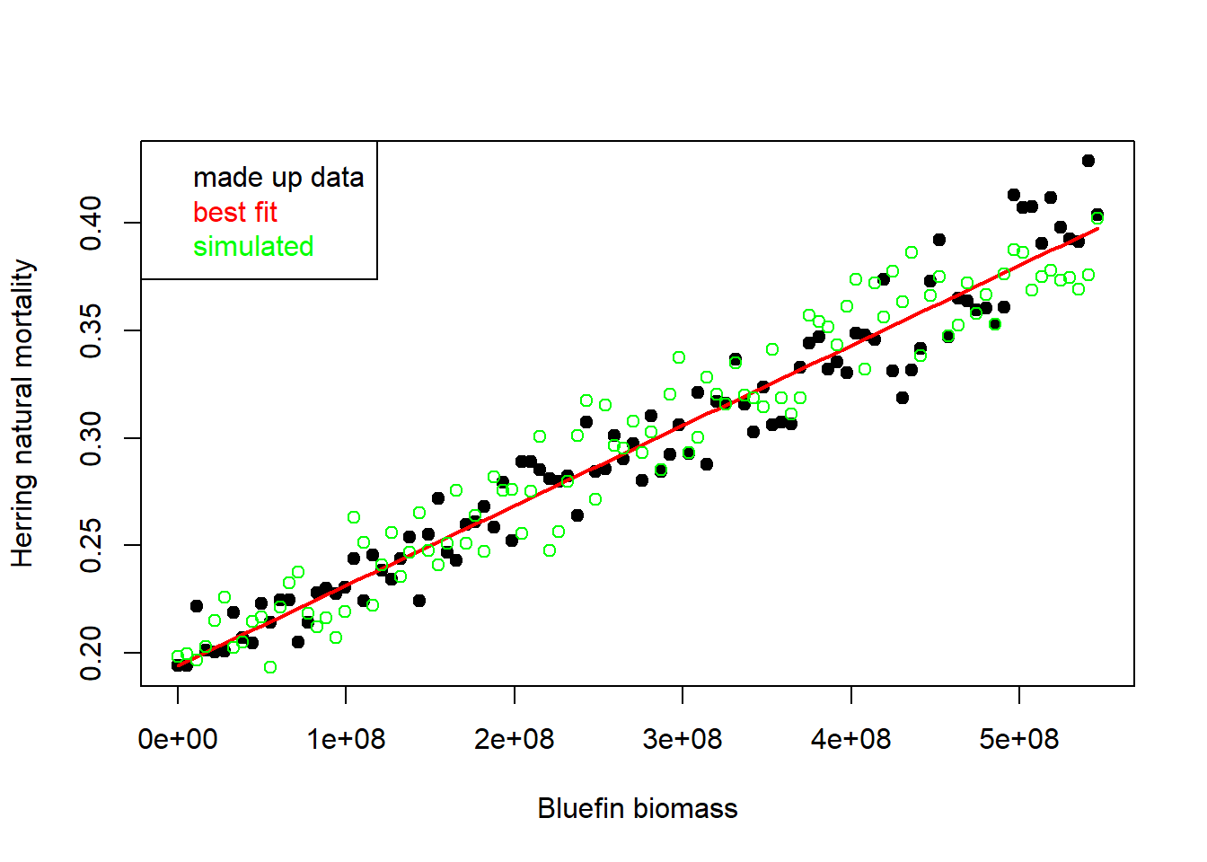
That is a lot to take in.
We derived a rough level of unfished bluefin biomass, made up some data (normally we would hope to have collected these) with log-normal error in herring M. We then fitted an R model (red line) and also demonstrated that we could use the simulate R function to simulate (green points) some new data based on that fit. Lastly, we placed our fitted model in a mysterious slot Rel.
Here are the important things to know about inter-stock relationships listed in the Rel slot:
Any R model can be used that:
- is compatible with the function
simulate - has specific coding for independent (e.g. the bluefin biomass) and dependent variables (e.g. the herring natural mortality rate)
The available options of independent variables are:
- B = total stock biomass
- SSB = total spawning stock biomass
- N = total stock numbers
- SSB0 = unfished spawning biomass
- B0 = unfished total biomass
- x = simulation number
The available options dependent variables are:
- M = Natural mortality rate (mature individuals by default, but can also be specified for a specific age class)
- K = von Bertalanffy growth parameter K
- Linf = asymtotic size Linf
- t0 = von Bertalanffy theoretical age at length-0
- a = weight length parameter a (\(W=aL^b\))
- b = weight length parameter b (\(W=aL^b\))
- Perr_y = recruitment deviation from the stock-recruit function
The terms in the R model should be denoted by the name of the variable, followed by underscore, then an integer that denotes the stock. So SSB_5 is the spawning stock biomass of the fifth stock in the Stocks slot, Linf_2 is the asymptotic length of stock 2 in the stocks slot.
Dependent values are calculated for year y+1 based on the value of the independent variables in year y. There is an exception for natural mortality for the duration of year y is determined by state variables at the beginning of y. An additional option is allowed specify whether the recruitment deivation for y+1 is determined by state variables in y+1 (within year effects) or from the previous year y (default, independent variable in year y affects the recruitment deviation in the following year y+1 (default) or within year y (see custom Rel).
There can be several inter-stock relationships for an operating model. However, within a single relationship, there can only be one dependent variable, but many independent variables:
M_3 ~ B_1 + B_2 - B_4You can’t have transformed independent variables but you can transform the dependent variables so this model is possible:
hs_3 ~ log(B_2) * log(B_1)but not this:
log(hs_3) ~ B_2 + B_1Intra-stock relationships are also possible! For example, a single stock operating model with a linearly density-dependent natural mortality relationship based on abundance would be:
M_1 ~ N_1And another thing, the order you place these in the Rel slot determines the order in which they operate. This may not be consequential yet, but plans are in the works to let an dependent variable in one relationship be the independent in the next.
The idea behind the Rel slot of the MOM object is to open up the option of including ecosystem driven relationships in a terse ‘models of intermediate complexity’ (MICE) format.
A note of caution before you go hog-wild with the Rel slot: it is probably fairly easy to set up a set of relationships and stock depletions that are impossible to solve in the initialization of the operating models in multiMSE. We haven’t had this issue yet, but do give some thought about the proposed relationships before you, for example, make herring M = 5 when bluefin depletion is 0.1 and then specify bluefin depletion as 0.1 and herring at 0.8…
After running the projections, the updated parameters can be viewed in the output object in MMSE@Misc$MICE.
Constructing the MOM Object
Now we have six lists:
- Stocks
- Fleets
- Obs
- Imps
- CatchFrac
- Rel
We can construct an object of class MOM:
MOM_BH <- new('MOM', Stocks, Fleets, Obs, Imps, CatchFrac, Rel = Rel, nsim = nsim)Single Stock MOM
If you wish to specify only a single stock but multiple fleets (e.g. just bluefin above) that is pretty easy:
Stocks <-    list( Bluefin_tuna )
Fleets <-    list( list(Generic_FlatE, Generic_IncE, Generic_DecE) )
Obs <-       list( list(Precise_Unbiased, Precise_Unbiased, Precise_Unbiased) )
Imps <-      list( list(Perfect_Imp, Perfect_Imp, Overages) )
CatchFrac <- list( matrix( rep(c(0.8,   0.01,   0.19), each=nsim), nrow=nsim) )

MOM_1S <- new('MOM', Stocks, Fleets, Obs, Imps, CatchFrac, nsim=nsim)
Stocks is just a list 1 stock object long. CatchFrac is a list 1 stock long of catch fractions by simulation and fleet. For any hierarchical list (Fleets, Obs, Imps) there is just one position (one stock) in which you have to place a list of Fleet, Obs and Imp objects.
Single Fleet MOM
If you want to model multiple stocks but are happy with aggregate fleet dynamics for each stock, that is fairly straight forward:
#                     Stock 1    Stock 2
Stocks <-    list( Bluefin_tuna, Herring )
#                         Bluefin                Herring
Fleets <-    list(  list(Generic_FlatE),    list(Generic_FlatE)    )
Obs <-       list( list(Precise_Unbiased), list(Imprecise_Biased) )
Imps <-      list(   list(Perfect_Imp),       list(Overages)      )

MOM_1F <- new('MOM', Stocks, Fleets, Obs, Imps, Rel = Rel, nsim=nsim)
Note we no longer have to specify CatchFrac as we do not have to calculate fleet-specific catchabilties using observed recent catch fractions.
A unique fleet for each stock
If you wish to model many stocks but in each case you are able to aggregate fleet dynamics (a single fleet), then you do exactly as above for the single fleet case but put a stock specific-fleet in position 1:
#                     Stock 1    Stock 2  Stock 3
Stocks <-    list( Bluefin_tuna, Herring, Mackerel )
#                         Bluefin fleet           Herring fleet       Mackerel fleet
Fleets <-    list(  list(Generic_FlatE),    list(Generic_IncE),     list(Generic_DecE)    )
Obs <-       list( list(Precise_Unbiased), list(Imprecise_Biased),  list(Precise_Biased) )
Imps <-      list(   list(Perfect_Imp),       list(Overages),       list(Overages)      )
CatchFrac <- list( matrix(1, nrow=nsim),   matrix(1, nrow=nsim),    matrix(1, nrow=nsim) )

MOM_FS <- new('MOM', Stocks, Fleets, Obs, Imps, CatchFrac, Rel = Rel, nsim=nsim)
One way or another we have our multi operating model, now we need some MPs to test …