Case study

Pacific cod example

In British Columbia, Canada, Pacific cod was assessed in 2018 with an update in 2020 (Forrest et al. 2020, DFO 2021). Here, data for Area 5ABCD (Hecate Strait and Queen Charlotte Sound) was used to condition operating models, which mimicked the configuration of the delay difference assessments.

Function call setup

The data and preliminary operating model for Pacific cod 5ABCD is available in SAMtool:

library(SAMtool)
data(pcod)

The base assessment had the following data and features:

Single fishing fleet with catch (pcod$data@Chist) and mean weight series (pcod$data@MS)
Five indices of abundance (pcod$data@Index)
Maturity and selectivity are knife-edge at age-two
Priors were set for several indices of abundance to inform stock size in the model
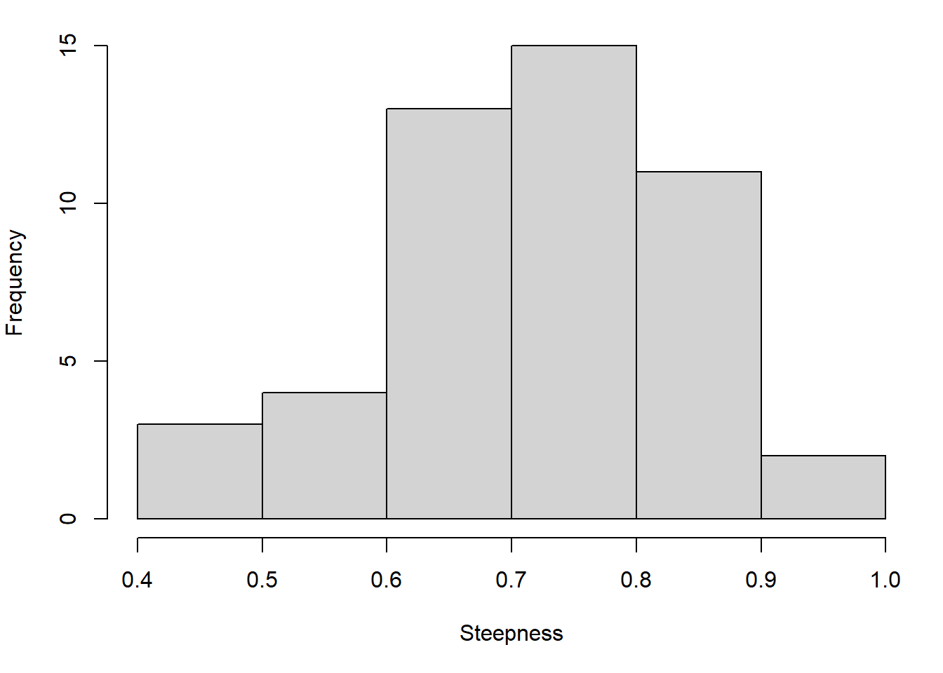
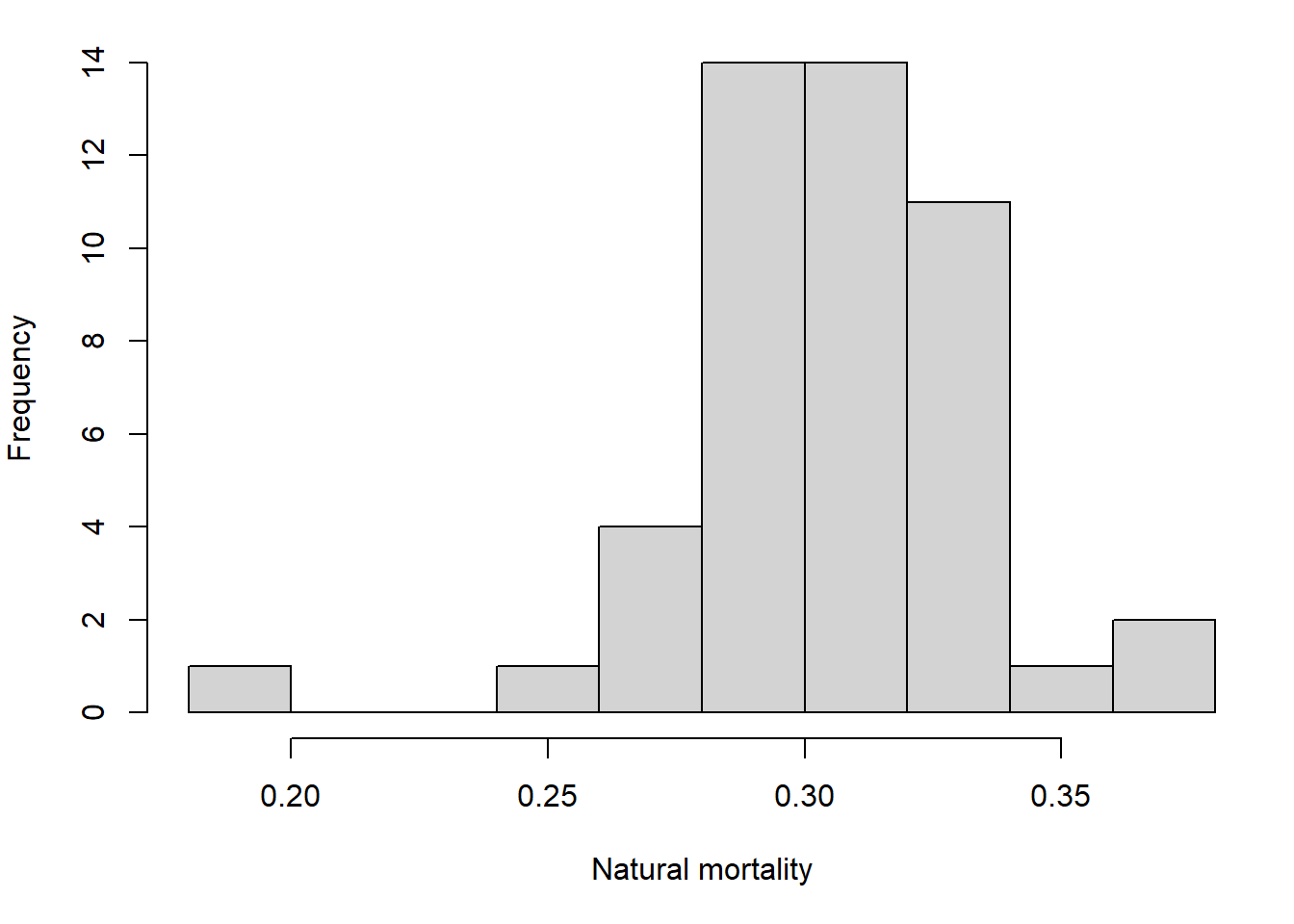
Priors were also set for stock-recruit steepness and natural mortality
Initial depletion entering the first year of the model (1956) was estimated as a deviation from equilibrium unfished recruitment

A function call of the conditioning model that incorporates these features looks like this:

mat_ogive <- ifelse(0:pcod$OM@maxage < 2, 0, 1)
out <- RCM(OM = pcod$OM, data = pcod$data, 
           condition = "catch", mean_fit = TRUE,
           selectivity = "free", s_selectivity = rep("SSB", ncol(pcod$data@Index)),
           start = list(vul_par = matrix(mat_ogive, length(mat_ogive), 1)),
           map = list(vul_par = matrix(NA, length(mat_ogive), 1),
                      log_early_rec_dev = rep(1, pcod$OM@maxage)),
           prior = pcod$prior)

Operating model

The preliminary operating model (pcod$OM) contains biological parameters for growth, maturity, natural mortality, steepness, recruitment variability that will be used to inform the conditioning model.

The operating models were set up with values of steepness pcod$OM@cpars$h and M pcod$OM@cpars$M sampled from their respective distributions, the means and standard deviations of which were informed by the posterior of the delay difference assessment.

Selectivity

See the article on setup of fleet and index selectivity here.

Knife-edge selectivity is set up by setting selectivity = "free" and providing the selectivity-at-age matrix in the vul_par argument. Since selectivity is fixed and not estimated, the map_vul_par argument is also provided (a matrix of NA).

Index selectivity is informed by the knife-edge maturity in the OM, so argument s_selectivity is set to "SSB" for all 5 indices.

Initial depletion

By default, the RCM generates an unfished population in the first year of the model, but we can estimate a deviation from unfished recruitment as a deviation from equilibrium unfished recruitment. A deviation log_early_rec_dev exists for each age cohort (of age-1 and older) in the first year of the model. To set them up as a single estimated parameter, we set the map argument to one for all these parameters map_log_early_rec_dev = rep(1, OM@maxage) (the map argument indicates to TMB whether parameter values are shared together or fixed to starting values).

Priors on catchability

Priors on index q can be set through pcod$prior <- list(q = ...) for two of the five indices, following the assessment:

pcod$prior$q

##                   Mean  SD
## HSMSAS              NA  NA
## SYN QCS     0.40820819 0.3
## SYN HS      0.06548742 0.3
## CPUE Hist           NA  NA
## CPUE Modern         NA  NA

Results

Model fits and estimated parameters can be found in the markdown reports:

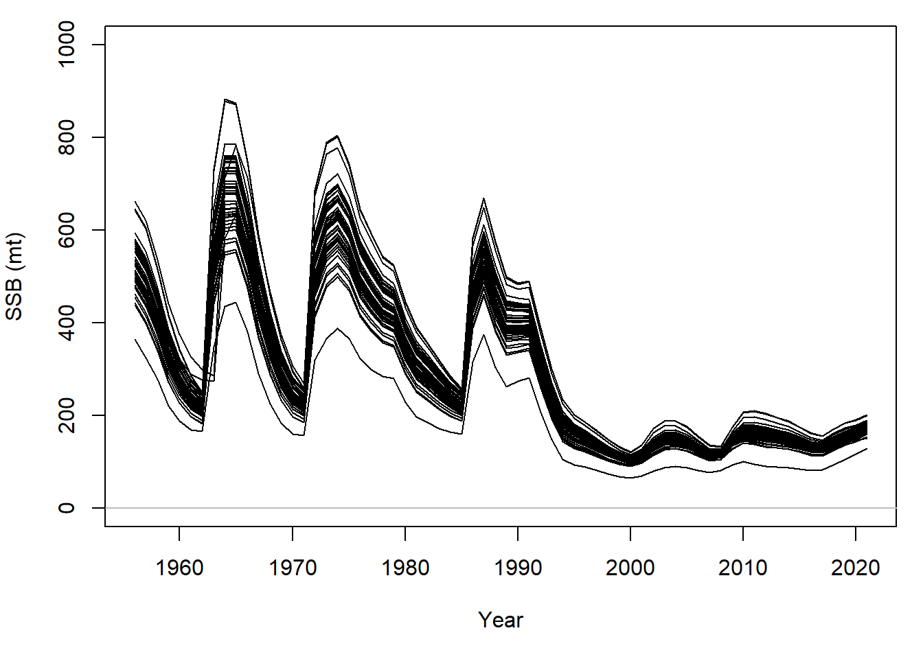
plot(out)

Since we sampled steepness and natural mortality from a distribution, a range of historical SSB values is reconstructed:

When conditioned on catch, a range for fishing mortality is similarly produced:

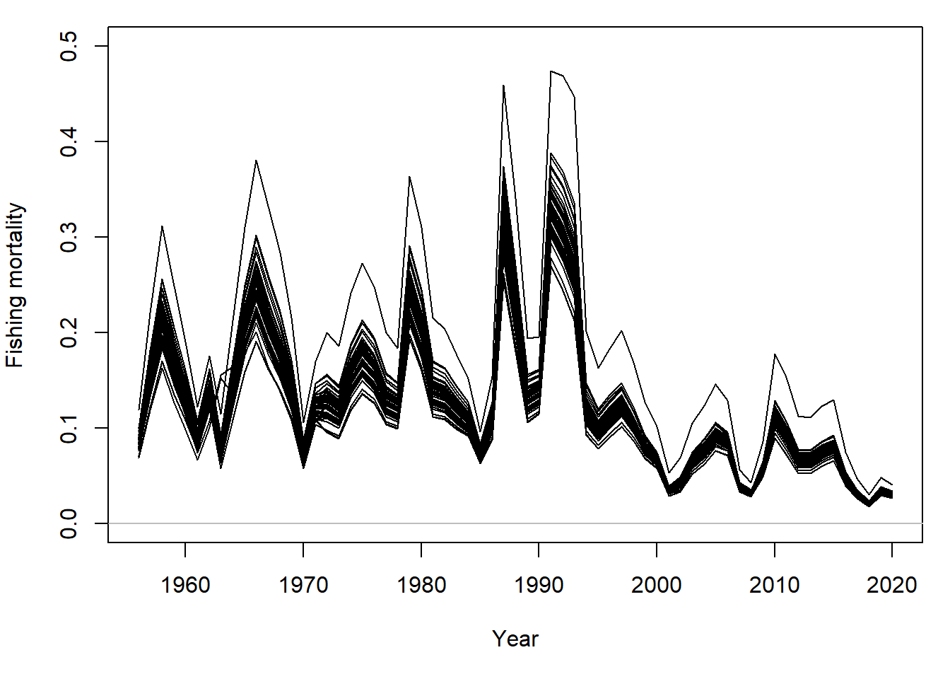
For all simulations, the SSB in 2020 is below the upper stock reference (USR), the mean SSB estimated during 1956-2004:

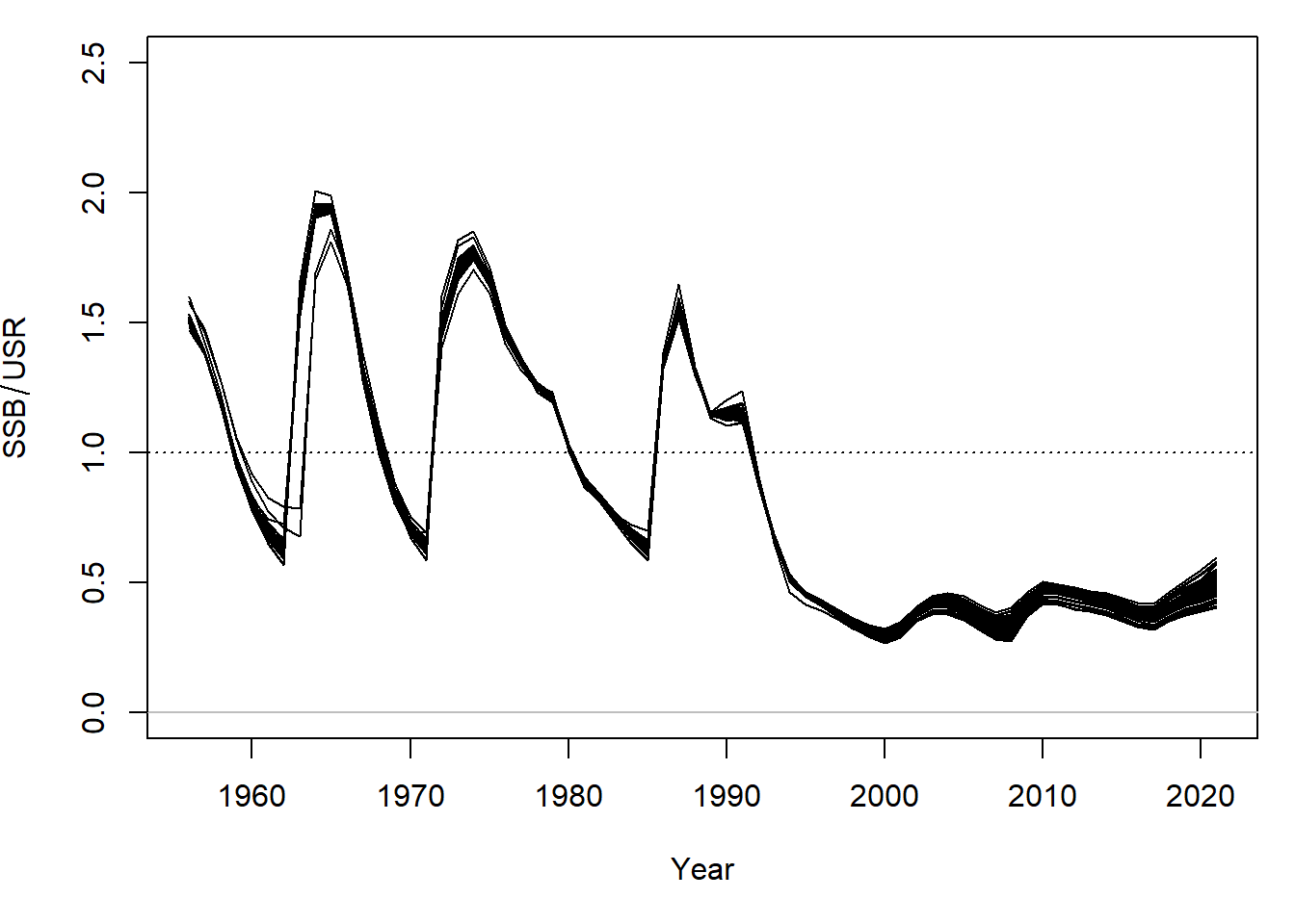
These figures are comparable to Figures 19, 20, and 22 of Forrest et al. 2020.

Finally, RCM also generates an updated OM that is ready for closed-loop simulation, where the historical period is conditioned by the estimation model:

MSE <- MSEtool::runMSE(out@OM, ...)

Alternative operating models

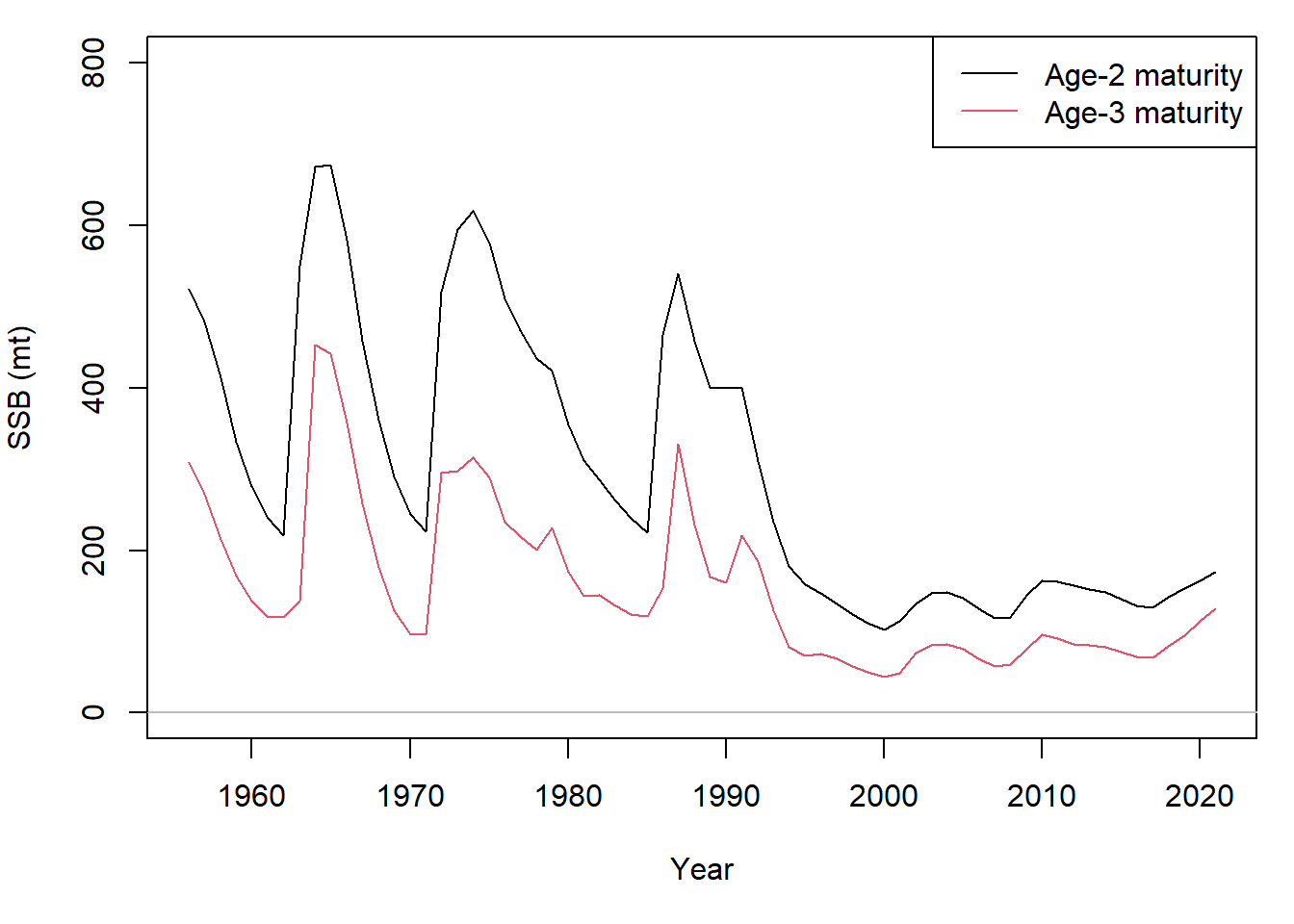
An alternative scenario can be generated where knife-edge maturity and selectivity is age-3 instead of age-2. The following code that updates the maturity and fishery/index selectivity in the OM and RCM:

out_age3 <- local({
  pcod$OM@cpars$Mat_age[, 3, ] <- 0
  mat_ogive_age3 <- pcod$OM@cpars$Mat_age[1, , 1]
  RCM(OM = pcod$OM, data = pcod$data, 
      condition = "catch", mean_fit = TRUE,
      selectivity = "free", s_selectivity = rep("SSB", ncol(pcod$data@Index)),
      start = list(vul_par = matrix(mat_ogive_age3, length(mat_ogive_age3), 1)),
      map = list(vul_par = matrix(NA, length(mat_ogive_age3), 1),   
                 log_early_rec_dev = rep(1, pcod$OM@maxage)),
      prior = pcod$prior)
})

Comparing multiple model fits

From multiple OM scenarios and corresponding RCM fits, the compare_RCM function allows users to compare RCM fits, estimated parameters, and likelihood values.

compare_RCM(out, out_age3, 
            scenario = list(names = c("Age-2 maturity", "Age-3 maturity")),
            s_name = colnames(pcod$data@Index))

The comparison primarily uses the mean scenarios from each OM: