Relative reference points such as \(\frac{B_\text{MSY}}{B_0}\), and \(\frac{SB_\text{MSY}}{SB_0}\) are calculated relative to the unfished biomass described in the previous section. This means that it is relatively straightforward to initialize the simulation model at a fraction of \(\text{SB}_\text{MSY}\) rather than \(\text{SB}_0\).
Depletion as fraction of SBMSY
For example, suppose you wish to set the depletion in the final historical year at \(0.5SB_\text{MSY}\):
OM <- testOM; OM@nsim <- 2
# need to populate OM@cpars$D so that random samples are the same
OM@cpars$D <- runif(OM@nsim, OM@D[1], OM@D[2])
Hist <- runMSE(OM, Hist=TRUE, silent=TRUE)
# update Depletion to 0.5 BMSY using cpars
OM@cpars$D <- 0.5 * Hist@Ref$ReferencePoints$SSBMSY_SSB0
Hist <- runMSE(OM, Hist=TRUE, silent=TRUE)

matplot(t(apply(Hist@TSdata$SBiomass, 1:2, sum)/Hist@Ref$ReferencePoints$SSBMSY),
        type="l", ylim=c(0,3),
        ylab="SB/SBMSY", xlab="Historical Years", bty="l")
abline(h=0.5, lty=2, col="gray")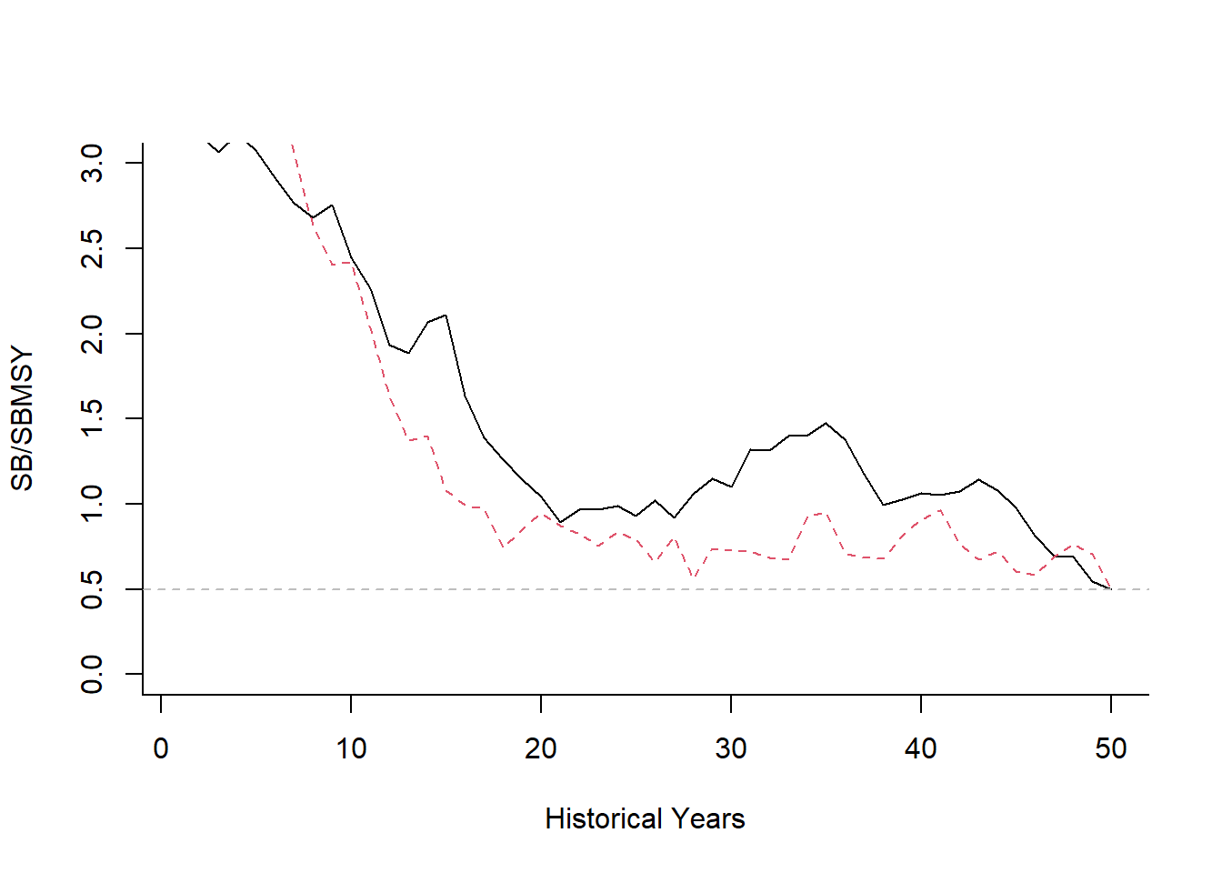
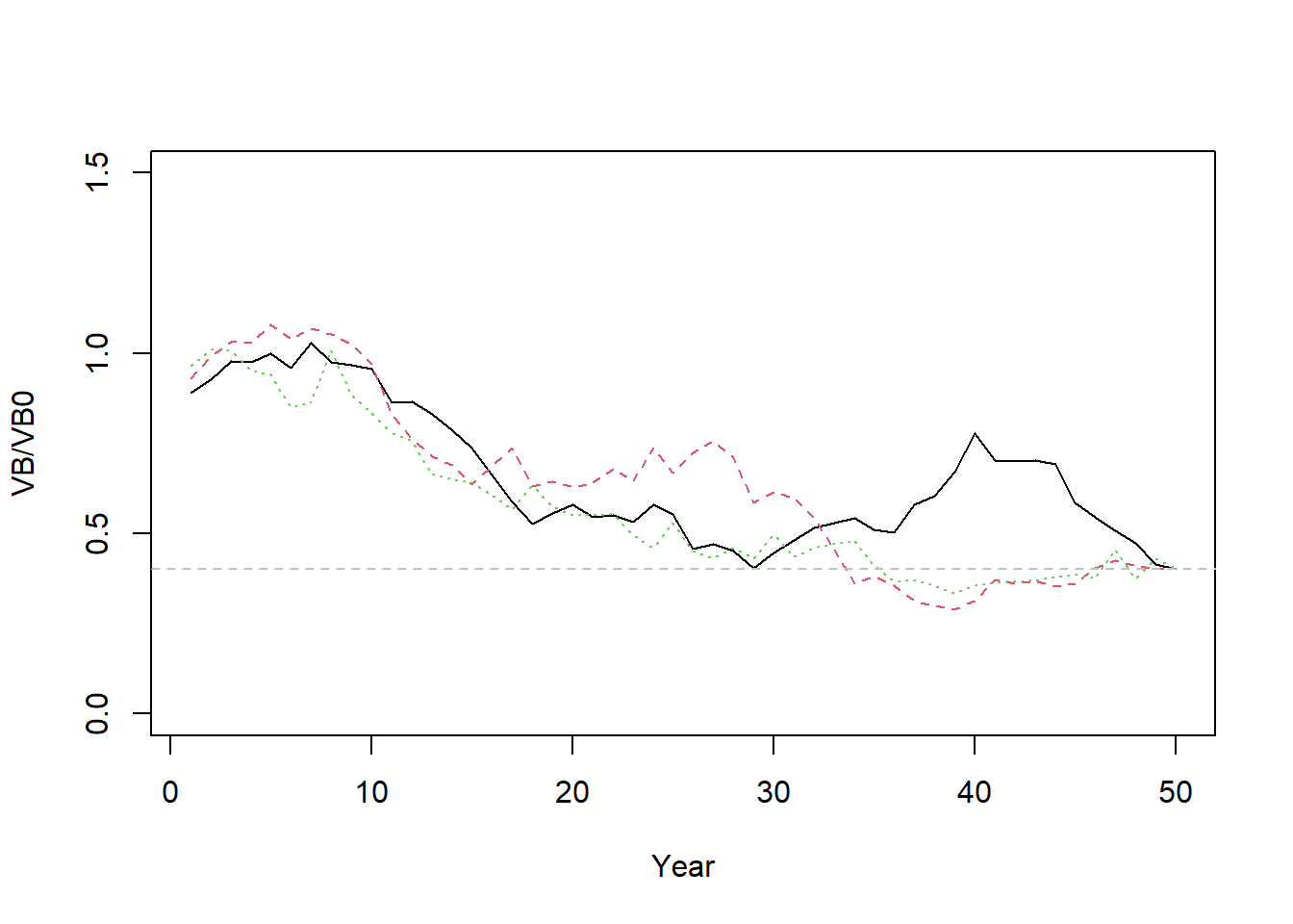
Depletion as fraction of VB0
The model can be modified to optimize for depletion in terms of average unfished vulnerable biomass (\(\text{VB}_0\)) rather than spawning biomass using the control Custom Parameters feature:
OM <- testOM
# switch to depletion in terms of VB0
OM@cpars$control$D <- 'VB'

# set depletion
OM@cpars$D <- rep(0.4, OM@nsim)
Hist <- Simulate(OM,silent=TRUE)

# VB time-series
VB <- apply(Hist@TSdata$VBiomass, 1:2, sum)

matplot(t(VB/matrix(Hist@Ref$ReferencePoints$VB0, nrow=OM@nsim, ncol=OM@nyears)),
        type="l", xlab="Year", ylab="VB/VB0", ylim=c(0,1.5))
abline(h=0.4, lty=2, col="gray")