Change in stock-recruit relationship

While the stock-recruit relationship is constant in openMSE, it is possible to change the effective stock-recruit relationship by changing the mean $\mu$ of the recruitment deviations through OM@cpars$Perr_y. This article describes how reference points implicitly change with $\mu$. The internal code used to calculate annual reference points in MSEtool::runMSE is not altered when the mean of OM@cpars$Perr_y is altered, so it is up to the user to decide whether reference points (see code below) need to be re-calculated.

Stock-recruit parameters

With the Beverton-Holt stock recruit relationship, the recruitment in year $y$ is:

\[ R_y = \dfrac{\alpha SB_y}{1 + \beta SB_y} \delta_y\]

where $\delta_y$ are recruitment deviates. For stationary productivity around the recruitment predicted by the S-R curve, we sample $\delta_y$ from a lognormal distribution with $E[\delta_y] = 1$ and $V[\delta_y] = \exp(\sigma^2-1)$. These values are passed to the operating model in OM@cpars$Perr_y. Parameters $\alpha$ and $\beta$, along with $\phi_0$, can be used to calculate the corresponding unfished recruitment $R_0$ and steepness $h$:

\[ h = \dfrac{\alpha \phi_0}{4 + \alpha \phi_0}\]

\[ R_0 = \dfrac{1}{\beta}\left(\alpha - \dfrac{1}{\phi_0}\right)\]

We define the unfished biomass as $SB_0 = R_0 \phi_0$. For easier reading, we have dropped the superscript $\textrm{SR}$ associated with $R_0$, $h$, and $\phi_0$.

If we want to change the productivity via recruitment deviations, we can re-scale the recruitment deviations. Set $\delta'_y = \mu \delta_y$, with $\mu < 1$ for a less productive system. In effect, we will have created a different stock-recruit relationship:

\[ R_y = \dfrac{\alpha SB_y}{1 + \beta SB_y} \delta'_y = \dfrac{\alpha' SB_y}{1 + \beta SB_y} \delta_y\]

where $\alpha' = \mu \alpha$, $E[\delta'_y] = \mu$ and $V[\delta'_y] = \exp(\sigma^2-1)/\mu^2$, and $\beta$ is unchanged. In other words, by setting the mean of OM@cpars$Perr_y to $\mu$, we create a stock-recruit relationship defined by $\alpha'$ and recruitment variance of $V[\delta'_y]$.

Implied reference points

Annual unfished and MSY reference points can be re-calculated accordingly with $\alpha'$, $\beta$, and $\phi_0$. The implications on the reference points can be seen in “new” parameters $R_0'$ and $h'$ corresponding to “new” $\alpha'$:

\[ h' = \dfrac{\alpha' \phi_0}{4 + \alpha' \phi_0} =\dfrac{\mu h}{1 + h (\mu - 1)}\]

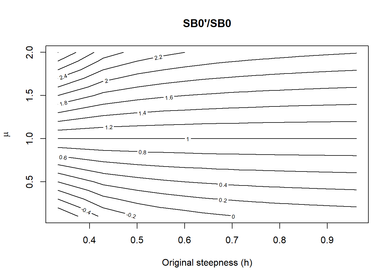
\[ R_0' = \dfrac{1}{\beta}\left(\alpha' - \dfrac{1}{\phi_0}\right) = R_0\dfrac{h(4\mu + 1) - 1}{5h-1}\] Then, $SB_0' = R_0' \phi_0$.

In the simplest case with constant $\phi_0$, we expect $h' < h$ and $R_0' < R_0$ when $\mu < 1$, and also expect $SB_0$, $F_{\textrm{MSY}}$, $\textrm{MSY}$, and $SB_\textrm{MSY}$ to decrease.

The new $SPR_{\textrm{crash}} = (\alpha'\phi_0)^{-1} = (\mu \alpha \phi_0)^{-1}$ increases ($F_{\textrm{crash}}$ decreases) when $\mu < 1$.

Examples

Contour plots

Let’s explore the ratio of the new and old values of $R_0$ and $h$ as a function of $\mu$ and the original steepness, with $\beta = 1$ and $\phi_0 = 1$:

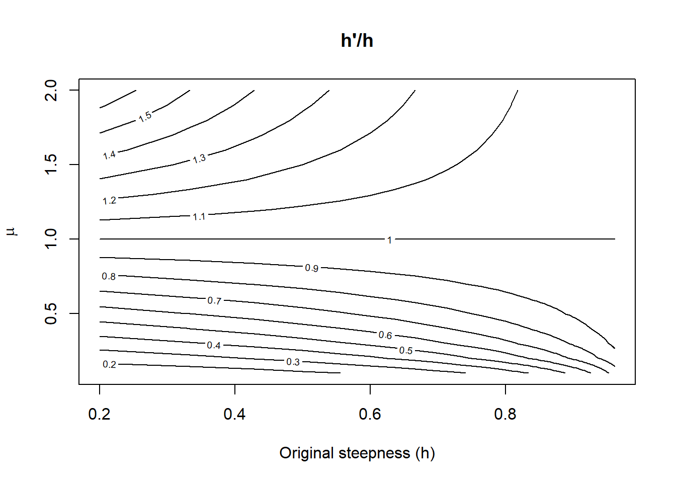
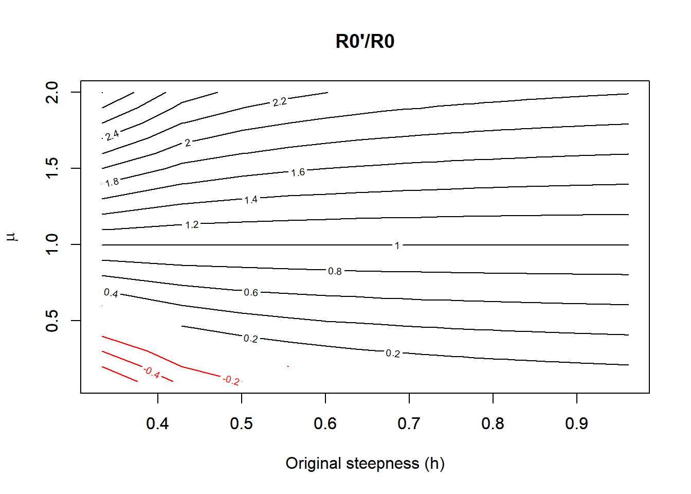
Interestingly, there can exist a combination of low steepness and low $\mu$ such that the population crashes, as implied by $R_0' \le 0$ in red.

Forward projections

Let’s explore the dynamics in a forward projecting model in MSEtool. We’ll create an operating model with 4 simulations with varying $\mu$ but constant stock-recruit parameters among simulations. Then we’ll project the model using the NFref (no fishing) MP.

library(MSEtool)

## Loading required package: snowfall

## Loading required package: snow

OM <- MSEtool::testOM

# Generate four simulations with same alpha, beta, and phi_0
OM@nsim <- 4
OM@Linfsd <- OM@Msd <- OM@Ksd <- c(0, 0)
OM@Linf <- mean(OM@Linf) |> rep(2)
OM@K <- mean(OM@K) |> rep(2)
OM@t0 <- mean(OM@t0) |> rep(2)
OM@M <- mean(OM@M) |> rep(2)
OM@L50 <- mean(OM@L50) |> rep(2)
OM@L50_95 <- mean(OM@L50_95) |> rep(2)
OM@h <- mean(OM@h) |> rep(2)

OM@Prob_staying <- OM@Frac_area_1 <- OM@Size_area_1 <- c(0.5, 0.5)

# With four simulations, let's set the projection Perr_y to these values:
mu_vec <- c(0.01, 0.75, 1, 1.5)
OM@cpars$Perr_y <- matrix(1, OM@nsim, OM@maxage + OM@nyears + OM@proyears)
OM@cpars$Perr_y[, OM@maxage + OM@nyears + 1:OM@proyears] <- mu_vec

Hist <- Simulate(OM, silent = TRUE)
MSE <- Project(Hist, MPs = "NFref", silent = TRUE)

Let’s see what happens with the NFref MP:

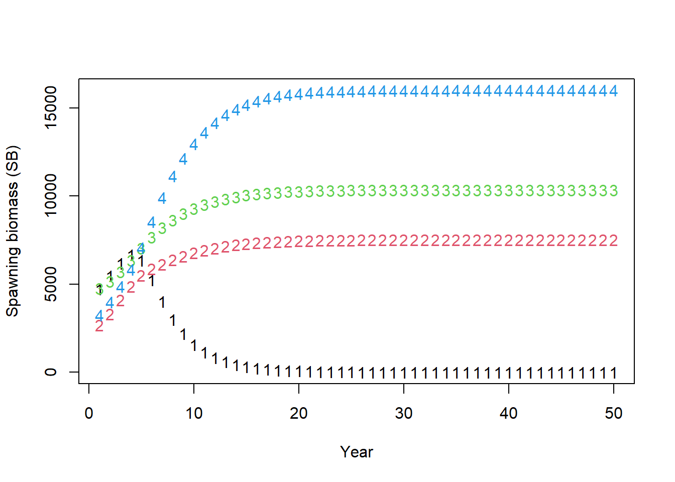
Despite the same stock-recruit parameters, the spawning biomass all diverge with $\mu$:

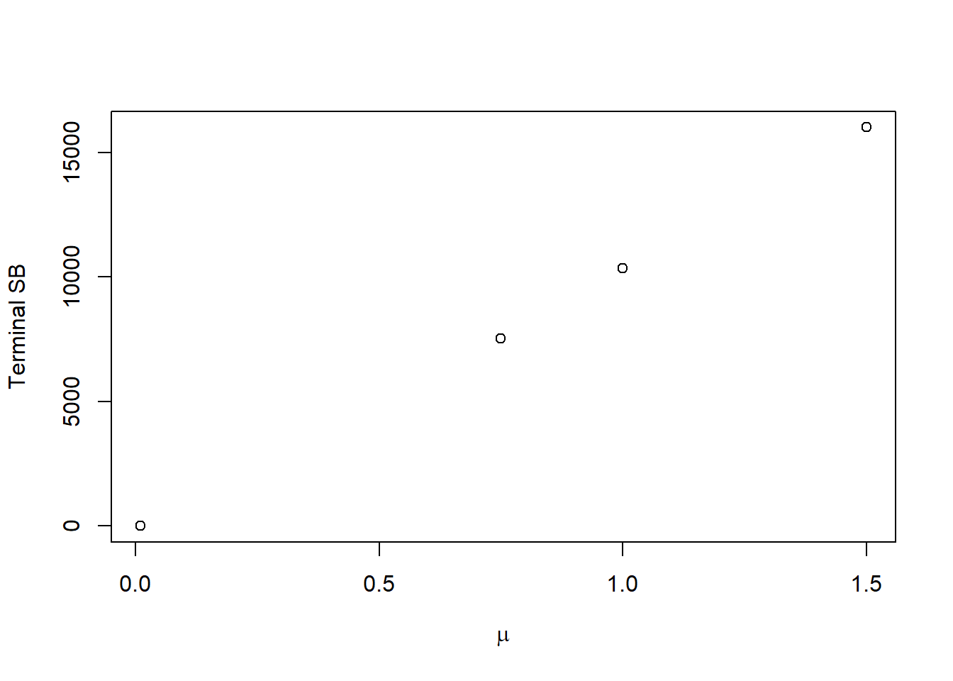
This terminal SB should be the new $SB_0$, so let’s create a function to calculate these values analytically instead of projecting:

recalc_ref_pt <- function(Hist, mu = rep(1, Hist@OM@nsim)) {
  StockPars <- Hist@SampPars$Stock
  FleetPars <- Hist@SampPars$Fleet
  R0 <- StockPars$R0
  hs <- StockPars$hs
  
  if(StockPars$SRrel[1] == 1) {
    R0_new <- R0 * (hs * (4 * mu + 1) - 1)/(5 * hs - 1)
    hs_new <- mu * hs /(1 + hs * (mu - 1))
  } else {
    R0_new <- 1 + 0.8 * R0 * log(mu)/log(5 * hs)
    hs_new <- hs * mu^0.8
  }
  
  MSY_ref_pt <- lapply(1:Hist@OM@nsim, function(x) { # Internal function for calculating unfished and MSY reference points
    sapply(Hist@OM@nyears + 1:Hist@OM@proyears, function(y) {
      MSEtool:::optMSY_eq(x, 
                          M_ageArray=StockPars$M_ageArray, 
                          Wt_age=StockPars$Wt_age, 
                          Mat_age=StockPars$Mat_age,
                          Fec_age=StockPars$Fec_Age, 
                          V=FleetPars$V_real, 
                          maxage=StockPars$maxage, 
                          R0=R0_new,
                          SRrel=StockPars$SRrel, 
                          hs=hs_new, 
                          SSBpR=StockPars$SSBpR,
                          yr.ind=y, 
                          plusgroup=StockPars$plusgroup)
    })
  })
  
  crash_ref_pt <- local({ # Internal function for calculating SPR crash
    boundsF <- c(1E-3, 3)
    F_search <- exp(seq(log(min(boundsF)), log(max(boundsF)), length.out = 50))
    
    lapply(1:Hist@OM@nsim, function(x) {
      sapply(Hist@OM@nyears + 1:Hist@OM@proyears, function(y) {
        Ref_search <- MSEtool:::Ref_int_cpp(F_search, 
                                            M_at_Age = StockPars$M_ageArray[x, , y],
                                            Wt_at_Age = StockPars$Wt_age[x, , y], 
                                            Mat_at_Age = StockPars$Mat_age[x, , y],
                                            Fec_at_Age = StockPars$Fec_Age[x, , y], 
                                            V_at_Age = FleetPars$V_real[x, , y],
                                            maxage = StockPars$maxage,
                                            plusgroup = StockPars$plusgroup)
        SPR_search <- Ref_search[2, ]
        RPS <- Ref_search[3, ]
        
        if(StockPars$SRrel[x] == 1) {
          CR <- 4 * StockPars$hs[x]/(1 - StockPars$hs[x])
        } else if(StockPars$SRrel[x] == 2) {
          CR <- (5 * StockPars$hs[x])^1.25
        }
        alpha <- mu[x] * CR/StockPars$SSBpR[x, 1] # New alpha
        
        if(min(RPS) >= alpha) { # Unfished RPS is steeper than alpha
          SPRcrash <- min(1, RPS[1]/alpha) # Should be 1
          Fcrash <- 0
        } else {
          SPRcrash <- MSEtool:::LinInterp_cpp(RPS, SPR_search, xlev = alpha)
          Fcrash <- MSEtool:::LinInterp_cpp(RPS, F_search, xlev = alpha)
        }
        c(SPRcrash = SPRcrash, Fcrash = Fcrash)
      })
    })
  })
  ref_pt <- abind::abind(simplify2array(MSY_ref_pt), simplify2array(crash_ref_pt), along = 1)
  dimnames(ref_pt)[[1]] <- c("MSY", "FMSY", "SBMSY", "SBMSY_SB0", "BMSY_B0", "BMSY", "VBMSY", "VBMSY_VB0", "RMSY", "SB0", "B0", "R0", "h",
                             "N0", "SN0", "SPRcrash", "Fcrash")
  return(ref_pt)
}

Let’s compare the ratio of the calculated $SB_0$ and the projected terminal SSB:

new_ref_pt <- recalc_ref_pt(Hist, mu = mu_vec)
SSB0_prime <- new_ref_pt["SB0", OM@proyears, ]
plot(mu_vec, SSB0_prime/terminal_SB, xlab = expression(mu), ylab = "SB0/Terminal SB")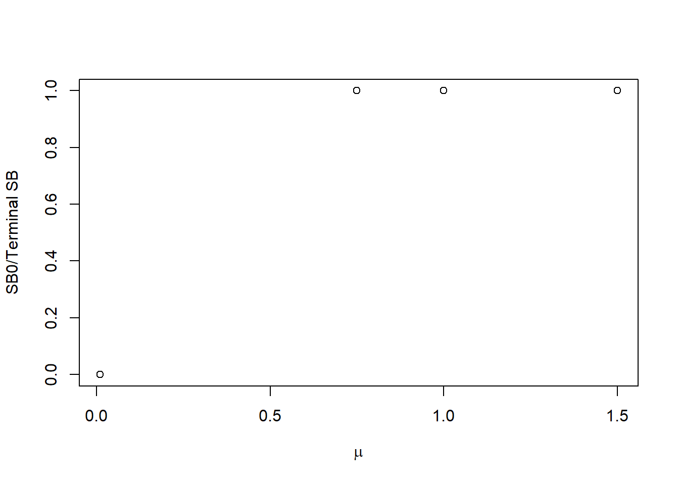

Looks like our new reference points match the values from the projections. Note with $\mu = 0.01$, the population crashes so $SB_0 = 0$.

Now let’s map out $h'/h$ and $R_0'/R_0$ as a function of $\mu$:

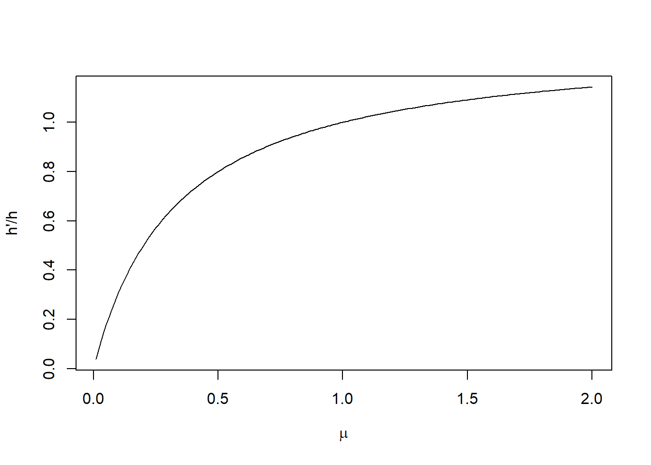
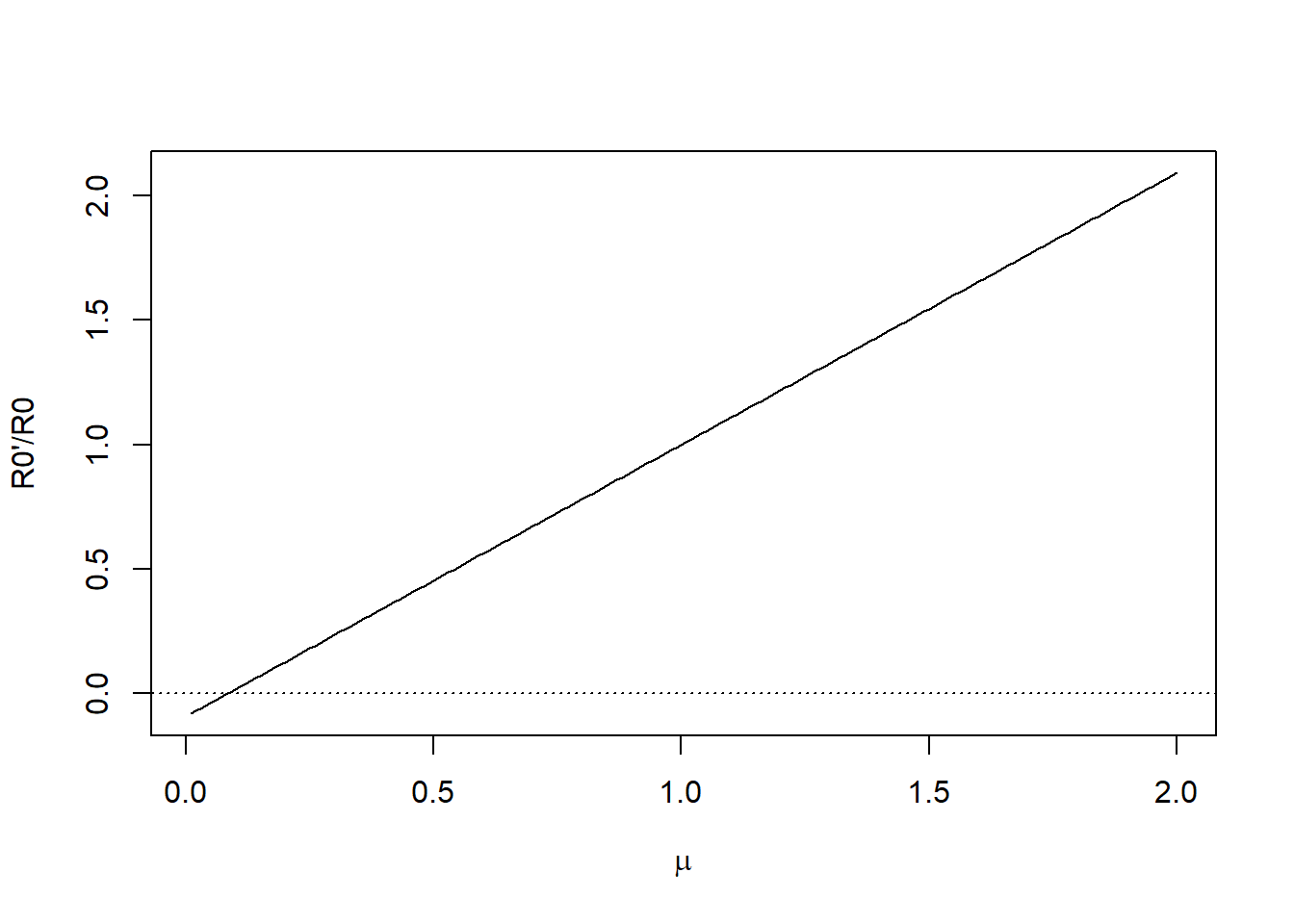
If $\mu < 0.08$, our population crashes because $R_0' < 0$, and $SPR_{\textrm{crash}} = 1$:

SPRcrash <- new_ref_pt["SPRcrash", OM@proyears, ]
plot(mu_vec, SPRcrash, xlab = expression(mu), ylim = c(0, 1))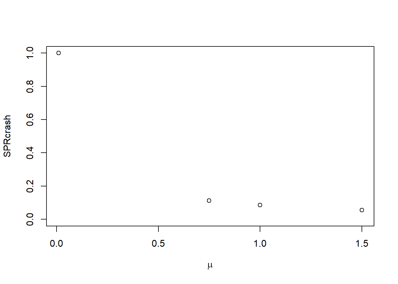

Ricker function

With a Ricker function where $R_y = \alpha SB_y \exp(-\beta SB_y) \delta_y$, steepness is $h = 0.2(\alpha\phi_0)^{0.8}$ and $R_0 = \log(\alpha\phi_0)/(\beta \phi_0)$.

The new SR relationship is $R_y = \alpha' SB_y \exp(-\beta SB_y) \delta_y$, with

\[h' = 0.2 (\alpha' \phi_0)^{0.8} = \mu^{0.8} h\]

\[R_0' = 1 + \dfrac{0.8 R_0\log(\mu)}{\log(5h)}\]