Ensuring Results are Reproducible

To ensure the simulations are consistent across machines, OM@seed is used to set the seed for the random number generator:

set.seed(OM@seed)

Sampling Custom Parameters

Next nsim values of the OM parameters are sampled from the operating model.

First, the Custom Parameters slot (OM@cpars) is sampled:

SampCpars <- SampleCpars(cpars=OM@cpars, OM@nsim)

## No valid names found in custompars. Ignoring `OM@cpars`

OM@cpars is not used in this operating model, so SampCpars is a empty list. If OM@cpars was populated with Valid Custom Parameters nsim samples of each custom parameter would be drawn from OM@cpars.

Correlations are maintained when sampling from OM@cpars.

Sampling OM Objects

Next, the Stock, Fleet, Obs, and Imp parameters are sampled from the OM:

StockPars <- SampleStockPars(OM, cpars=SampCpars)

## Note: Maximum age ( 23 ) is lower than assuming 1% of cohort survives 
## to maximum age ( 32 )

## Optimizing for user-specified movement

FleetPars <- SampleFleetPars(OM, StockPars, cpars=SampCpars)
ObsPars <- SampleObsPars(OM, cpars=SampCpars, Stock=StockPars)
ImpPars <- SampleImpPars(OM, cpars=SampCpars)

A few things to notice here:

• There is a message alerting us that OM@maxage is lower than the age where about 1% of a cohort would survive to. This is usually not a problem because the model groups all age-classes beyond OM@maxage into a plus-group. But given there is little computational cost in increasing maximum age, users may wish to set OM@maxage <- 32 so that more age-classes are explicitly modeled.

• SampCpars is provided to each of the functions that sample the Stock, Fleet, Obs, and Imp parameters. Parameters that are included in the Custom Parameters are used and these parameters are not sampled from the OM object.

• StockPars contains the biological parameters for the spool-up and projection periods, e.g., StockPars$M_ageArray is an array with M-at-age with dimensions c(OM@nsim, OM@maxage+1, OM@nyears+OM@proyears).

• FleetPars contains the exploitation parameters for the spool-up period (e.g, FleetPars$Find) and the selectivity/retention parameters for the spool-up and projection period, e.g., FleetPars$V is an array with vulnerability-at-age with dimensions c(OM@nsim, OM@maxage+1, OM@nyears+OM@proyears). The selectivity and retention parameters may be updated in the projection period if an MP changes the selectivity/retention pattern.

• ObsPars contains the observation parameters for all years (e.g., ObsPars$Cobs_y) is a matrix with dimensions c(OM@nsim, OM@nyears+OM@proyears) with catch observation error.

• ImpPars contains the implementation error for the projection years; e.g., ImpPars$TAC_y is a matrix with dimensions c(OM@nsim, OM@proyears) with TAC implementation error.

Calculate Unfished Reference Points

The unfished reference points are calculated by running the simulation model with no fishing mortality and no recruitment deviations.

The equilibrium unfished reference points are calculated for each year. For example, the annual unfished spawning stock biomass (SSB0) is calculated for the 75 historical years and the 40 projection years:

matplot(t(Hist@Ref$ByYear$SSB0), type="l", xlab="Year", ylab="SSB0", lwd=2)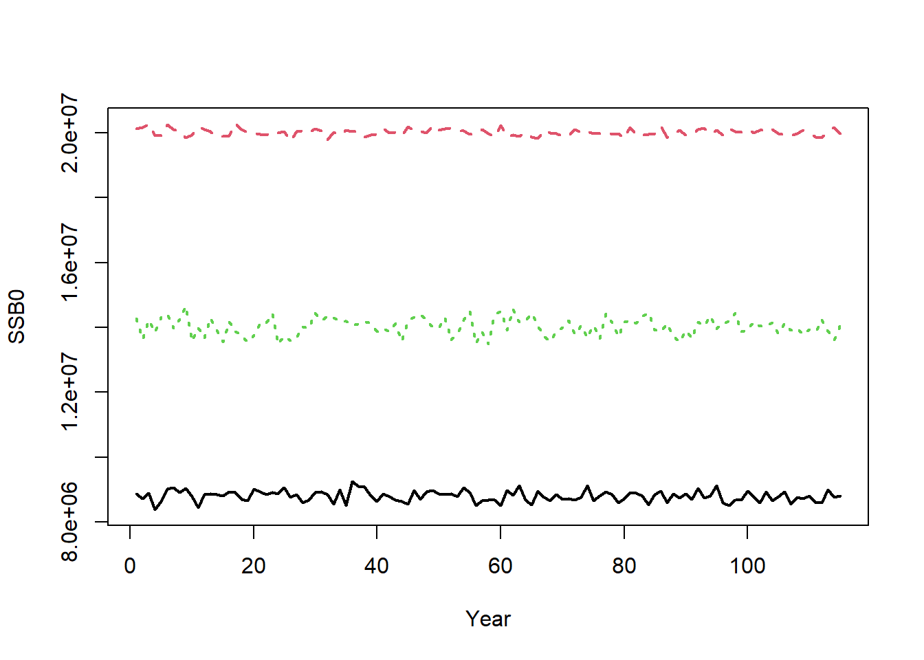

The small amount of inter-annual variability in SSB0 is caused by inter-annual variability in the life-history parameters (e.g., OM@Msd). The inter-annual variability in SSB0 would be greater if there was more variability in OM@Msd, OM@Linfsd, and OM@Ksd.

The SSB0 used to determine depletion is calculated by averaging Hist@Ref$ByYear$SSB0 over several years. See Depletion and Unfished Reference Points for details.

Dynamic unfished reference points (i.e., including recruitment deviations) are also calculated and returned in Hist@Ref$Dynamic_Unfished. For example, the dynamic unfished spawning stock biomass is:

matplot(t(Hist@Ref$Dynamic_Unfished$SSB0), type="l", xlab="Year",
        ylab="Dynamic SSB0", lwd=2)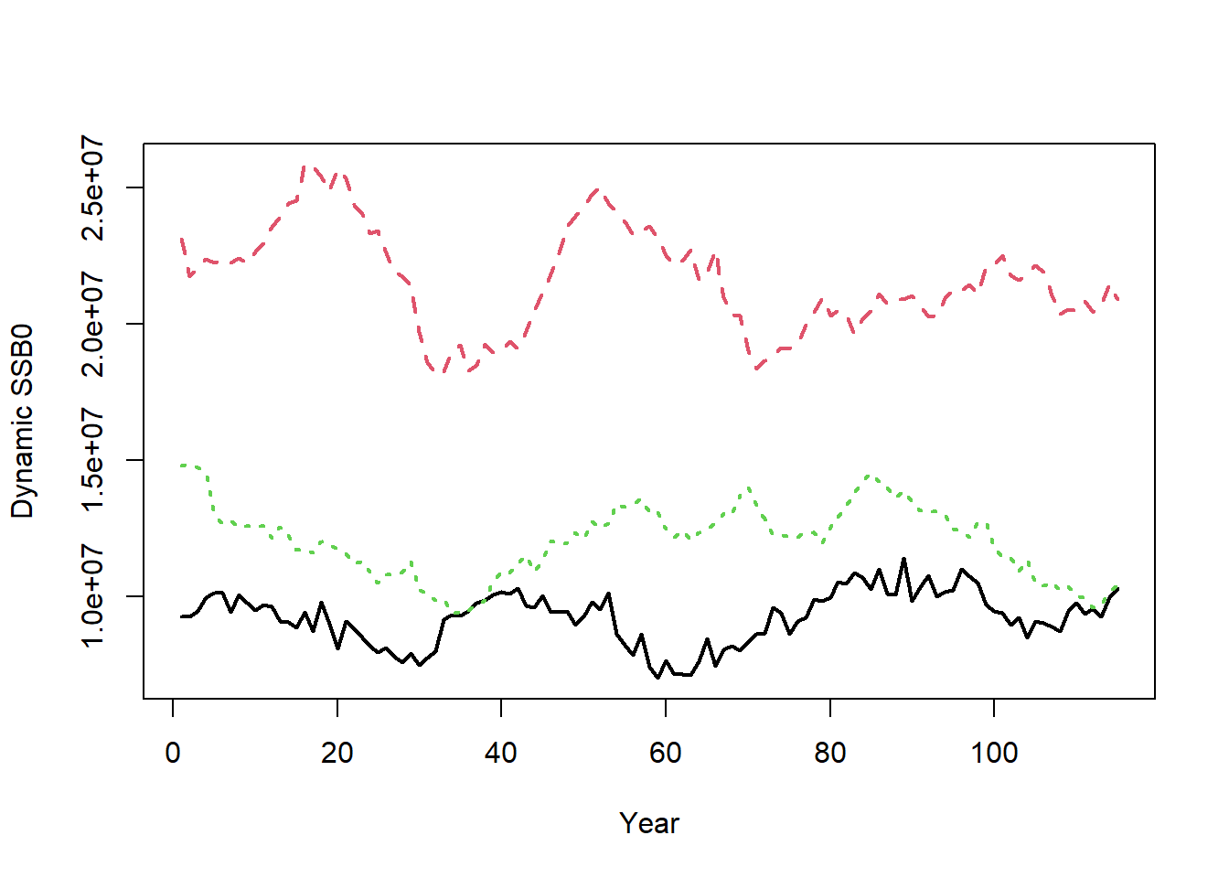

Calculate MSY Reference Points

Maximum sustainable yield (MSY) reference points are calculated using the information in StockPars and FleetPars. MSY reference points are calculated in each year, assuming equilbrium conditions (no recruitment deviations) and the life-history and selectivity parameters in each year.

For example,

matplot(t(Hist@Ref$ByYear$MSY), type="l", xlab="Year", ylab="MSY", lwd=2)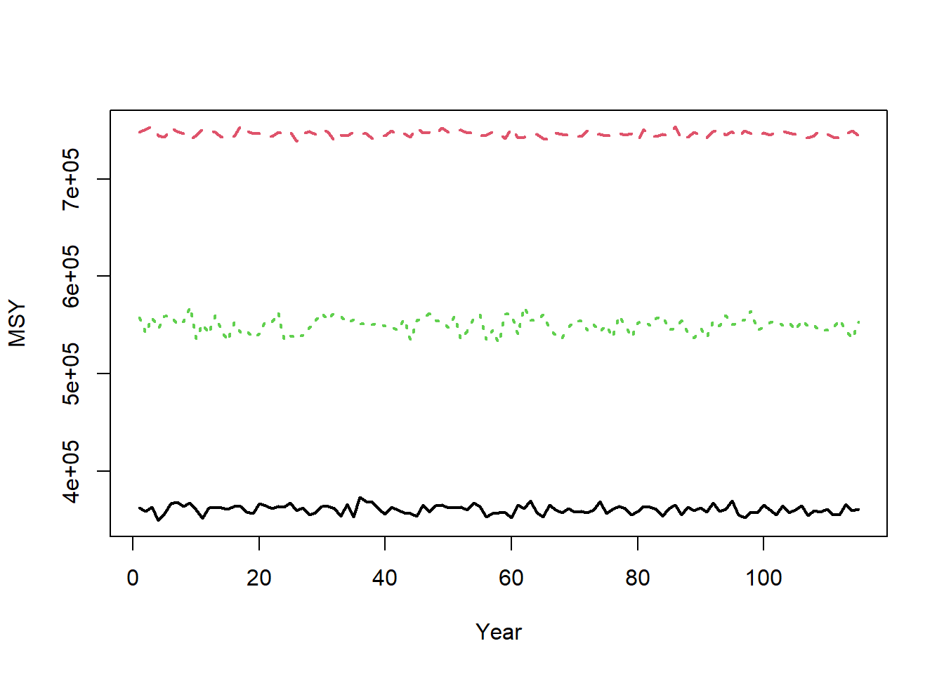

See MSY Reference Points for more details.

Optimize for Depletion

openMSE was designed to allow easy access to MSE modeling for data-limited fisheries. By definition, historical fishing mortality and current depletion is not known in a data-limited fishery.

Instead, the general pattern in fishing mortality is specified in the Fleet Object and a range of depletion values in the Stock Object (or in Custom Parameters if distributions other than uniform are required).

For each simulation, the model uses the relevant parameters (relative pattern in fishing mortality, size-at-age in each year, selectivity, recruitment deviations, etc) and optimizes for the catchability coefficient q so that the depletion at the end of the spool-up period matches the value drawn from OM@D.

We demonstrate with an example for a single simulation:

sim <- 1
# Depletion value for this simulation
Hist@SampPars$Stock$Depletion[sim]

## [1] 0.06173859

# SSB time-series (sum over areas)
SSB <- rowSums(Hist@TSdata$SBiomass[sim,,])

# SSB0 for this sim
SSB0 <- Hist@Ref$ReferencePoints$SSB0[sim]

plot(1:OM@nyears, SSB/SSB0, ylim=c(0, 1), lwd=2, 
     xlab="Year", ylab="Depletion (SB/SB0)", type="l", las=1,
     bty="n")
abline(h=Hist@SampPars$Stock$Depletion[sim], lty=3)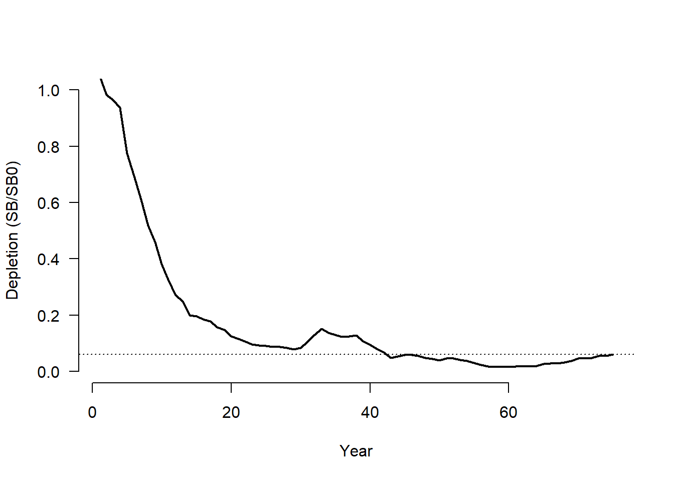

Stocks where historical fishing mortality and depletion are known can skip this step by specifying the apical fishing mortality in OM@cpars$Find and setting catchability coefficient to 1 (OM@cpars$qs <- rep(1, OM@nsim)). See Custom Fleet Parameters for more details.

Calculate Reference Yield

Reference yield is calculated by projecting the population forward from the end of the spool-up period for OM@proyears with a fixed F policy and optimizing for the F that results in the highest long-term yield.

In other words, reference yield is the highest yield obtainable for a given set of OM parameters under a policy of constant fishing mortality.

Reference yield is returned in Hist@Ref$ReferencePoints$RefY. It is usually reasonably close to MSY (i.e., Hist@Ref$ReferencePoints$MSY) but as MSY is an equilibrium value, it does not account for the impact of recruitment deviations in the simulations.

Reference yield can be useful for standardizing the yield outcomes of management procedures. In data-limited fisheries, the OM is often scale-less (i.e., OM@R0 is in arbitrary units) and absolute yield outcomes may not be meaningful.

Yield relative to reference yield can be more useful. If your management procedure results in yield outcomes that are close to reference yield, it means it is performing (in terms of long-term yield at least) pretty close to the optimal fixed-F policy. Can’t do a lot better than that!

Calculate Catch and Removals

Catch is calculated using the Baranov equation (i.e., assuming continuous fishing):

\[ C_y = \frac{F_y}{Z_y} N_y(1-e^{-Z_y})\]

Generate Data

Fishery data is generated by applying the observation model to the simulated fishery dynamics (e.g., simulated true catches, etc).

If the OM has been conditioned with data the Data Object provided in OM@cpars$Data will be used in the simulations. See Conditioning OMs with Data for more details.